JoeGuardian Automation

8. Analog Output Architecture in Studio 5000 — Setpoints, Limits, Scaling, and Safe Commands

In the previous article, we followed an analog signal from a field transmitter into the PLC:

Field Instrument
      ↓
Analog Input Module
      ↓
Raw / Channel Data
      ↓
Scaling
      ↓
Engineering Units
      ↓
Validation
      ↓
Process Value

Now we will reverse the direction.

Instead of receiving an analog value from the process, the PLC will generate an analog command and send it to a field device.

Typical analog output applications include:

• VFD speed reference
• Control valve position
• Proportional pressure regulator
• Damper position
• Heater power reference
• Pump speed command
• Flow-control command
• Analog actuator position

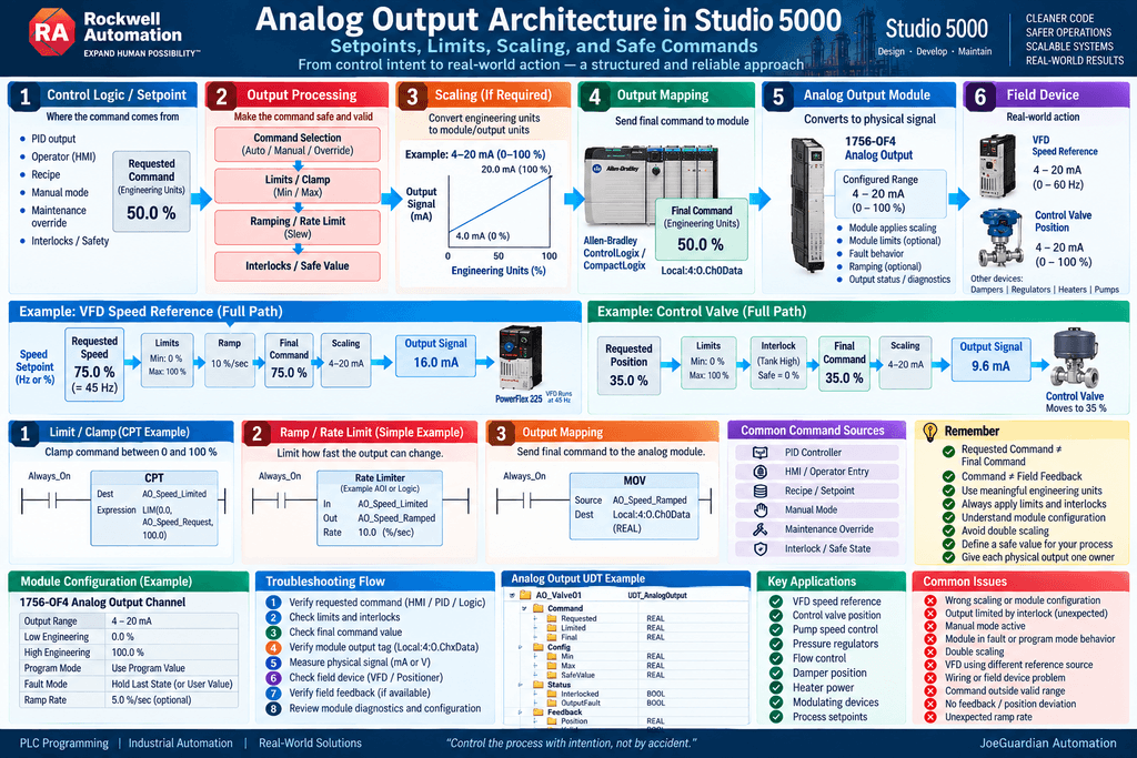
A robust analog output architecture should not simply write a number directly to the module.

A better design considers:

Control Setpoint
      ↓
Command Selection
      ↓
Limits / Clamp
      ↓
Ramp / Rate Limit
      ↓
Engineering Units
      ↓
Output Mapping
      ↓
Analog Output Module
      ↓
4–20 mA / 0–10 V
      ↓
Field Device

The goal is to ensure that the value leaving the PLC is:

intentional, valid, limited, traceable, and safe for the process.

What Is an Analog Output?

A digital output typically has two states:

0 = OFF
1 = ON

An analog output represents a continuously variable command.

For example:

0–100 %

may represent:

Valve Position

or:

VFD Speed Reference

The physical output signal may be:

4–20 mA

or:

0–10 VDC

depending on the module and field device.

Example: VFD Speed Reference

Suppose a conveyor VFD accepts:

4–20 mA

for speed reference.

The engineering meaning is:

4 mA  = 0 %
20 mA = 100 %

The PLC may calculate:

VFD01.Command.SpeedRef = 60.0 %

The analog output system then produces the corresponding physical signal.

Conceptually:

60 %
 ↓
Analog Output Processing
 ↓
13.6 mA
 ↓
VFD

If the VFD maximum speed is:

60 Hz

then:

60 % = 36 Hz

assuming a linear relationship.

Example: Control Valve

A modulating valve might use:

4 mA  = 0 % Open
20 mA = 100 % Open

The PLC could command:

Valve01.Command.Position = 35 %

The output system sends the corresponding signal.

The architecture becomes:

Process Controller
       ↓
35 % Valve Command
       ↓
Analog Output
       ↓
Valve Positioner
       ↓
Valve Moves

Command vs Physical Signal

This distinction is extremely important.

The application logic should ideally think in meaningful engineering units:

Valve Position = 35 %

rather than:

Output = 9.6 mA

or some hardware-specific raw number.

The software should describe the process.

The I/O layer should handle the hardware relationship.

A Clean Analog Output Architecture

A practical architecture might be:

CONTROL LOGIC
      ↓
ENGINEERING COMMAND
      ↓
LIMITS
      ↓
RAMPING
      ↓
OUTPUT VALUE
      ↓
MODULE-DEFINED OUTPUT DATA
      ↓
ANALOG OUTPUT MODULE
      ↓
FIELD SIGNAL
      ↓
FIELD DEVICE

This separates:

What the process wants

from:

How the hardware produces it

Start With Engineering Units

Suppose a VFD speed reference uses:

0–60 Hz

The application could work directly in:

Hz

For example:

VFD01.Command.Speed = 42.0 Hz

Alternatively, a project may standardize command values as:

0–100 %

For example:

VFD01.Command.SpeedPct = 70.0

Either approach can work.

The key is consistency and clarity.

Percent vs Engineering Units

For some devices:

0–100 %

is the most natural representation.

Examples:

Valve Position
Damper Position
Heater Demand

For others, real engineering units may be more useful.

Examples:

VFD Speed = 45 Hz
Pressure Setpoint = 60 PSI
Flow Command = 120 GPM

The application should use the representation that best matches the process.

Limit the Command Before Sending It

Suppose an operator enters:

Speed Command = 150 %

Should the PLC send that directly to the analog output?

No.

A good output architecture includes limits.

For example:

Minimum Command = 0 %
Maximum Command = 100 %

Then:

150 %

becomes:

100 %

before it reaches the hardware.

This is commonly called:

Clamping

What Is Clamping?

Clamping keeps a value inside an allowed range.

Conceptually:

Command < Minimum
       ↓
Use Minimum

Command within range
       ↓
Use Command

Command > Maximum
       ↓
Use Maximum

For example:

Min = 0
Max = 100

If:

Command = -15

then:

Limited Command = 0

If:

Command = 125

then:

Limited Command = 100

Why Limits Matter

Limits protect against:

• Bad HMI entries
• Calculation errors
• Incorrect recipes
• Invalid PID outputs
• Startup conditions
• Communication problems
• Programming mistakes

They also document the expected operating range.

Process Limits May Be Narrower Than Hardware Limits

This is important.

A valve may physically support:

0–100 %

but the process may only allow:

20–80 %

during normal operation.

Likewise, a pump may support:

0–60 Hz

but engineering may require:

Minimum = 20 Hz
Maximum = 55 Hz

The software limit should represent the real process requirement.

Minimum Speed Example

Consider a cooling-water pump controlled by a VFD.

Physical range:

0–60 Hz

But the pump should not operate continuously below:

20 Hz

because of cooling, lubrication, or process requirements.

The command architecture might therefore use:

Requested Speed
       ↓
If Run Command = 1
Clamp between 20 and 60 Hz
       ↓
Output Speed

This prevents an invalid operating condition.

Do Not Confuse Clamp With Interlock

A clamp limits a numeric value.

For example:

80 Hz → 60 Hz

An interlock decides whether operation is permitted.

For example:

Low Tank Level
       ↓
Pump Interlocked
       ↓
Speed Command = Safe Value

These are different concepts.

Interlocks and Analog Outputs

Analog outputs need interlock behavior just like digital outputs.

Suppose a control valve normally receives:

Valve01.Command.Position = 70 %

Then a critical interlock becomes active.

The desired response may be:

Valve Position → 0 %

or:

Valve Position → 100 %

or:

Hold Last Value

depending on the process.

There is no universal safe analog value.

Safe Value Is Process-Specific

This is crucial.

For one valve:

Safe = 0 %

For another:

Safe = 100 %

For another:

Safe = Hold Last Position

The correct behavior depends on:

• Process hazard
• Valve fail position
• Equipment design
• Safety analysis
• Control philosophy

Never assume:

Analog output fault = force zero.

That may be wrong for the process.

Rockwell Process Analog Output

Modern Rockwell process architectures provide the Process Analog Output (PAO) instruction.

Rockwell documents that PAO can manage analog output commands, scale engineering units to output units, monitor I/O fault conditions, handle operator/program command sources, apply ramping, and force configured output behavior during interlocks.

Conceptually, this is exactly the architecture we are building:

Command
 ↓
Mode / Source Selection
 ↓
Limits / Interlocks
 ↓
Ramping
 ↓
Scaling
 ↓
Output

Important: The Module May Already Use Engineering Units

This is where Studio 5000 differs from the simplified idea that every analog output must be manually converted into raw counts.

For supported 1756 analog output modules operating in floating-point mode, Rockwell documents:

Ch0Data

as a REAL representing the requested output value in configured engineering units. The module then applies that value according to its configuration, limits, program mode, calibration state, and ramping behavior.

That means a configured module may allow the PLC to write something like:

Local:4:O.Ch0Data = 50.0

where:

50.0

already means:

50 %

if the channel has been configured that way.

Module-Level Scaling

For certain ControlLogix analog output modules, the module configuration allows you to define relationships such as:

Low Signal
High Signal
Low Engineering
High Engineering

Rockwell notes that values sent to and from these modules can be represented in engineering units after configuration.

For example:

4 mA  → 0 %
20 mA → 100 %

could be configured at the module level.

Then the PLC might simply write:

50.0

to request:

50 %

The module handles the electrical conversion.

Avoid Double Scaling

This creates the same warning we discussed for analog inputs.

Suppose the module is already configured:

0 EU   = 4 mA
100 EU = 20 mA

and the PLC writes:

50.0

The module understands:

50 %

If the PLC manually converts 50% into some raw value first and then writes that value into an engineering-unit channel, the output may be completely wrong.

Therefore:

Understand the module configuration before writing custom scaling logic.

When Manual Scaling Is Needed

Manual scaling may still be appropriate when:

• The module expects raw data
• A device uses a communication register rather than a traditional AO module
• The architecture standardizes internal commands differently
• A gateway expects a particular numeric range
• Custom scaling is required
• Legacy hardware uses integer formats

Then the familiar scaling equation applies.

Reverse Scaling Formula

For an analog output, we may convert engineering units into an output range.

The general formula is:

Output =
(Command - EUMin)
×
(OutputMax - OutputMin)
/
(EUMax - EUMin)
+
OutputMin

Example:

Engineering Range = 0–100 %
Output Signal      = 4–20 mA

For:

Command = 50 %

we get:

Output = 12 mA

Example Calculation

Given:

Command = 75 %

EUMin = 0
EUMax = 100

OutputMin = 4
OutputMax = 20

Then:

Output =
(75 - 0)
×
(20 - 4)
/
(100 - 0)
+
4

which becomes:

75 × 16 / 100 + 4

and:

12 + 4 = 16 mA

Therefore:

75 % = 16 mA

VFD Example

Suppose:

0 %   = 0 Hz
100 % = 60 Hz

and the VFD receives:

4–20 mA

A command:

VFD01.Command.SpeedPct = 75 %

represents:

45 Hz

and electrically:

16 mA

The architecture can therefore be visualized as:

75 %
 ↓
45 Hz
 ↓
16 mA
 ↓
VFD

But again, depending on the I/O module configuration, the PLC may only need to send the engineering-unit value.

Application Tag vs Module Tag

A good architecture does not require the process logic to directly manipulate:

Local:4:O.Ch0Data

throughout the program.

Instead:

VFD01.Command.Speed

or:

AO_VFD_Speed

can represent the application command.

Then the output mapping layer handles:

Application Command
        ↓
Module Output Tag

Example Output Mapping

Suppose:

AO_VFD_Speed_Command

is a REAL.

Output mapping may conceptually use:

MOV
Source: AO_VFD_Speed_Command
Dest:   Local:4:O.Ch0Data

if the data representation matches.

This creates a clear hardware boundary.

Analog Output UDT

Just like analog inputs, analog outputs can benefit from structured data.

For example:

UDT_AnalogOutput

could contain:

Request
Command
Limited
Output
SafeValue

Min
Max

ManualEnable
ManualValue

Interlocked
Faulted

Then:

Valve01

might contain:

Valve01.Request
Valve01.Command
Valve01.Output
Valve01.Interlocked

A More Structured Example

For a modulating valve:

Valve01.Command.Requested
Valve01.Command.Limited
Valve01.Command.Final

Valve01.Config.Min
Valve01.Config.Max
Valve01.Config.SafeValue

Valve01.Status.Interlocked
Valve01.Status.OutputFault

This creates excellent troubleshooting visibility.

Requested vs Final Command

This distinction is very useful.

Suppose:

Requested = 85 %

but:

Maximum Allowed = 70 %

Then:

Final = 70 %

During troubleshooting, the technician can immediately see:

Requested = 85
Limited   = 70
Final     = 70

instead of wondering why the field device refuses to move to 85%.

Manual Mode

Analog outputs often need manual control.

For example:

Automatic Command = 42 %
Manual Command    = 60 %

Then:

Manual Mode = 0

selects:

42 %

while:

Manual Mode = 1

selects:

60 %

The architecture becomes:

Automatic Command ──┐
                    ├── Source Selection
Manual Command ─────┘
                           ↓
                        Limits
                           ↓
                     Final Command

Manual Does Not Mean Unprotected

This is an important rule.

Manual mode should not automatically bypass:

• Safety requirements
• Critical equipment protection
• Required interlocks
• Hard process limits

Depending on the control philosophy, manual mode may bypass some automatic sequencing while still respecting protective logic.

Command Priority

More advanced systems may have multiple possible command sources:

Program
Operator
Maintenance
Override
Hand

Rockwell’s PAO instruction explicitly provides multiple operating and command-source modes for this reason.

A mature architecture should clearly define:

Who currently owns the analog output?

Ramping

Imagine changing a VFD command instantly:

20 Hz → 60 Hz

The process may not tolerate such a rapid change.

A ramp limits the rate at which the output changes.

For example:

5 Hz / second

Then:

20
25
30
35
40
...
60 Hz

instead of an immediate jump.

Why Ramp an Analog Output?

Ramping can reduce:

• Mechanical shock
• Pressure spikes
• Flow disturbances
• Valve hunting
• Product instability
• Sudden motor acceleration

Some Rockwell analog output architectures and process instructions include configurable ramping capabilities.

Do Not Duplicate VFD Ramping Blindly

A VFD may already have its own:

Acceleration Time
Deceleration Time

If the PLC also heavily ramps the speed reference, the two ramps interact.

That is not necessarily wrong.

But it should be intentional.

You should know whether the desired dynamic response is controlled by:

PLC ramp

or:

VFD accel/decel

or both.

Slew Rate / Rate Limiting

A general architecture may include:

Requested Command
       ↓
Clamp
       ↓
Rate Limit
       ↓
Final Command

For example:

Requested = 100 %

Maximum Rise Rate = 10 % / second

The command gradually moves toward 100%.

This is often called:

• Ramp
• Slew limit
• Rate limit

depending on the system.

Output Fault Behavior

The analog output module may also have configured behavior for conditions such as:

Program Mode
Fault Mode
Communication Failure

Rockwell’s module configuration supports defining output states and related behavior for certain 1756 analog modules.

These settings are part of the control design.

Do not assume the PLC program alone determines what happens when communication is lost.

Program Mode

Suppose the controller leaves Run mode.

What should the analog output do?

Possible configured behaviors may include:

Hold Last State

or:

Go to User-Defined Value

depending on hardware and configuration.

For a valve, this decision may significantly affect the process.

Communication Failure

Similarly, if the output module loses communication with the controller, the module may have configured fault behavior.

This must align with the process philosophy.

The question is:

What should the field device do when the controller can no longer command it?

That decision belongs in the design phase, not after a failure occurs.

Command vs Feedback

Just like digital motor control:

Command ≠ Feedback

If the PLC commands:

Valve Position = 70 %

that does not prove the valve actually reached:

70 %

A separate position transmitter may provide:

Valve01.Feedback.Position = 63 %

Now the PLC can compare:

Command = 70 %
Feedback = 63 %

Position Deviation

If:

|Command - Feedback|

exceeds an allowed tolerance for too long, the PLC can generate:

Position Deviation Alarm

Example:

Command = 70 %
Feedback = 40 %

after sufficient travel time.

Possible causes:

• Valve stuck
• Positioner fault
• Air pressure problem
• Mechanical binding
• Analog output problem
• Feedback transmitter problem

Output Echo Is Not Field Feedback

This distinction is critical.

Some Rockwell analog output modules provide echoed output data.

Rockwell documents the echoed value as useful for verifying communication and module behavior, but it does not by itself verify the actual field-side device position.

In other words:

PLC requested 50 %
Module echoes 50 %

does not necessarily mean:

Valve actually moved to 50 %

For real field confirmation, use actual device feedback when required.

Analog Output Troubleshooting Chain

Suppose a valve will not open beyond 30%.

A structured troubleshooting path is:

PROCESS REQUEST
      ↓
AUTOMATIC SETPOINT
      ↓
MANUAL / AUTO SOURCE
      ↓
LIMITS
      ↓
INTERLOCKS
      ↓
RAMP
      ↓
FINAL COMMAND
      ↓
MODULE OUTPUT TAG
      ↓
ANALOG MODULE
      ↓
4–20 mA
      ↓
FIELD WIRING
      ↓
POSITIONER
      ↓
VALVE
      ↓
POSITION FEEDBACK

Each stage can be checked individually.

Example Troubleshooting

Suppose:

Requested Position = 80 %

but the valve remains at:

30 %

Check:

1. Requested Command

Valve01.Command.Requested

Is it really 80%?

2. Limits

Valve01.Config.Max

Is the command being clamped?

3. Interlock

Valve01.Status.Interlocked

Is an interlock forcing another value?

4. Final Command

Valve01.Command.Final

What value is the output architecture actually requesting?

5. Module Output

Local:4:O.Ch0Data

Does it match the expected command?

6. Physical Signal

Measure:

4–20 mA

at the output loop.

7. Positioner

Does the valve positioner show the same demand?

8. Mechanical Device

Is the valve physically capable of moving?

9. Feedback

Does actual position agree with command?

That is far more effective than immediately replacing the analog output card.

VFD Troubleshooting Example

Suppose:

Speed Command = 50 Hz

but the motor runs at:

30 Hz

Check:

PLC Requested Speed
       ↓
PLC Final Speed
       ↓
AO Module Value
       ↓
Physical mA Signal
       ↓
VFD Analog Input Value
       ↓
VFD Reference Source
       ↓
VFD Minimum / Maximum Frequency
       ↓
VFD Speed Command
       ↓
Motor Speed

The problem may not be in the PLC at all.

Analog Output and PID

A common analog output source is a PID controller.

For example:

Pressure PV
      ↓
PID
      ↓
Control Output
      ↓
Valve Position

The PID might produce:

0–100 %

That value should still pass through the output architecture.

For example:

PID Output
    ↓
Limits
    ↓
Interlocks
    ↓
Final Command
    ↓
Analog Output

The PID should not necessarily have unrestricted ownership of the physical output.

Bumpless Transfer

When switching between:

Automatic

and:

Manual

an abrupt command jump may disturb the process.

A mature analog architecture may therefore use:

Bumpless Transfer

so the new command source starts near the current output.

This is especially important in process-control applications.

Simulation

Analog outputs can also be simulated.

During simulation:

Valve01.Command.Final

may continue to calculate normally while:

Physical Output Write

is disabled.

Instead, a simulated process model may consume the command.

Conceptually:

Final Analog Command
        ↓
     Selector
      /     \
REAL OUTPUT  SIMULATION MODEL

This allows testing without energizing real field hardware.

Maintenance Overrides

Maintenance may require forcing an output to a known value.

For example:

Maintenance Override = 25 %

A structured architecture should make this explicit:

Auto Command
Manual Command
Maintenance Command
Interlock Command

rather than hiding overrides inside scattered MOV instructions.

One Final Owner

As with digital outputs:

One final software value should own each analog output channel.

Avoid:

Routine A writes Local:4:O.Ch0Data
Routine B writes Local:4:O.Ch0Data
Routine C writes Local:4:O.Ch0Data

This becomes extremely difficult to troubleshoot.

A better pattern is:

Multiple command sources
        ↓
Command arbitration
        ↓
ONE final command
        ↓
ONE output mapping point
        ↓
Physical analog output

Example UDT

A practical analog output structure might be:

UDT_AnalogOutput

Command.Requested    REAL
Command.Manual       REAL
Command.Final        REAL

Config.Min           REAL
Config.Max           REAL
Config.SafeValue     REAL
Config.RampRate      REAL

Status.Interlocked   BOOL
Status.Faulted       BOOL
Status.Manual        BOOL

Feedback.Value       REAL
Feedback.Valid       BOOL

Diagnostic.Deviation BOOL

Then:

FCV101

could represent one flow-control valve.

Example Flow-Control Valve

The controller requests:

FCV101.Command.Requested = 68 %

Configuration:

FCV101.Config.Min = 0 %
FCV101.Config.Max = 100 %
FCV101.Config.SafeValue = 0 %

No interlock exists.

Final command:

FCV101.Command.Final = 68 %

Then:

FCV101.Command.Final
       ↓
Local:4:O.Ch0Data

assuming the module’s channel scaling is configured for 0–100 engineering units.

Interlock Example

Now suppose:

Tank_HighHigh = 1

requires the inlet valve to close.

Then:

FCV101.Status.Interlocked = 1

and:

FCV101.Command.Final = 0 %

The application can still retain:

Requested = 68 %

while clearly showing:

Final = 0 %

because of the interlock.

This is excellent for troubleshooting.

Do Not Overwrite the Reason

This is an important architecture principle.

Instead of simply changing:

Requested = 68

to:

Requested = 0

when an interlock occurs, preserve:

Requested = 68
Final = 0
Interlocked = 1

Now the technician can see:

The control system wanted 68%, but the interlock forced the final output to 0%.

That is far more informative.

Complete Analog Output Architecture

A mature architecture can look like:

┌──────────────────────────────┐
│ Automatic Command            │
│ PID / Sequence / Recipe      │
└──────────────┬───────────────┘
               ↓
┌──────────────────────────────┐
│ Command Source Selection     │
│ Auto / Manual / Maintenance  │
└──────────────┬───────────────┘
               ↓
┌──────────────────────────────┐
│ Clamp / Min / Max            │
└──────────────┬───────────────┘
               ↓
┌──────────────────────────────┐
│ Interlock / Safe Value       │
└──────────────┬───────────────┘
               ↓
┌──────────────────────────────┐
│ Ramp / Rate Limit            │
└──────────────┬───────────────┘
               ↓
┌──────────────────────────────┐
│ Final Engineering Command    │
└──────────────┬───────────────┘
               ↓
┌──────────────────────────────┐
│ Output Mapping               │
└──────────────┬───────────────┘
               ↓
┌──────────────────────────────┐
│ Analog Output Module         │
└──────────────┬───────────────┘
               ↓
┌──────────────────────────────┐
│ 4–20 mA / 0–10 V            │
└──────────────┬───────────────┘
               ↓
┌──────────────────────────────┐
│ VFD / Valve / Actuator       │
└──────────────────────────────┘

Practical Rules

Rule 1

Keep control logic in meaningful engineering units whenever practical.

Rule 2

Know whether the analog module expects raw data or engineering units.

Rule 3

Never assume custom scaling is required.

Rule 4

Avoid double scaling.

Rule 5

Clamp commands to valid ranges.

Rule 6

Define the correct process-safe interlock value.

Rule 7

Do not assume zero is always safe.

Rule 8

Separate:

Requested

from:

Final

command values.

Rule 9

Give each physical output channel one clear final owner.

Rule 10

Remember:

Command ≠ Field Feedback

Rule 11

Understand controller, module, and field-device fault behavior.

Rule 12

Document the complete relationship:

Engineering Command
Physical Signal
Field Device Range
Safe Value

Final Thought

Analog output architecture is not simply:

MOV Setpoint Local:4:O.Ch0Data

A well-designed output system answers:

Who is requesting the command?

What are the valid limits?

Is an interlock active?

What is the final command?

How fast may the output change?

What should happen during a fault?

What does the module actually expect?

Did the field device actually respond?

The goal is to transform:

Control Intent

into:

Safe, Predictable Field Action

That is the real purpose of a strong analog output architecture.

Next Article

PLC I/O Mapping Performance — Which Method Is Best for the Processor?

In the next article, we will compare:

Direct I/O
Alias Tags
Individual Mapping
MOV
COP
CPS
UDT-Based Mapping

from another perspective:

Controller performance

We will discuss:

• Scan-time impact
• Memory usage
• Mapping overhead
• COP vs individual instructions
• CPS synchronization cost
• Large UDT considerations
• Fast periodic tasks
• High-speed machinery
• When optimization actually matters
• Why maintainability usually matters more than saving a few instructions
• How to measure instead of guessing

The question will no longer be:

Which architecture looks cleaner?

Instead:

When does I/O architecture actually affect PLC performance?