9. PLC I/O Mapping Performance — Which Method Is Best for the Processor?
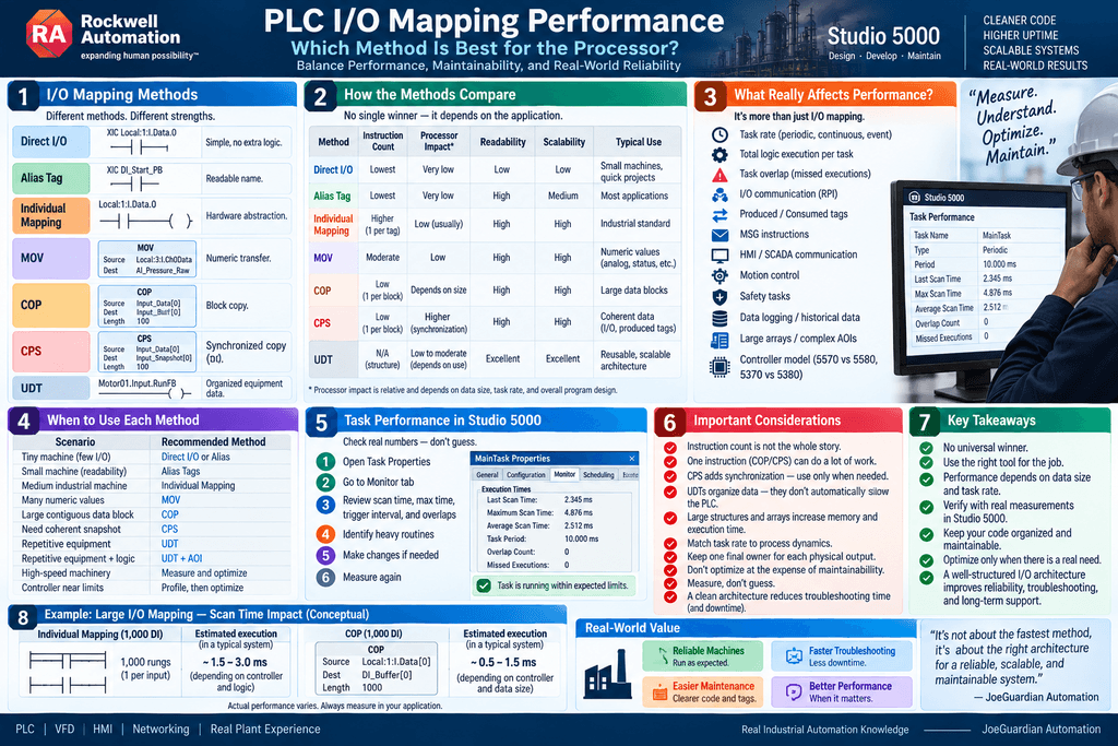
Throughout this series, we have examined several ways to build an I/O architecture in Studio 5000:
Direct I/O
Alias Tags
Individual Mapping
MOV
COP
CPS
UDTs
Each method offers different architectural advantages.
But eventually someone asks:
Which method is fastest?
Or:
Which method uses less PLC processor?
These are valid questions.
However, they are often asked too early.
For most industrial machines, the difference between a few Boolean mapping instructions and direct I/O references is not what determines whether the controller performs well.
A much better question is:
Is my I/O architecture creating a measurable performance problem?
That distinction matters.
PLC Performance Is More Than Scan Time
When technicians discuss PLC performance, they often think only about:
Scan TimeBut a Logix controller may also be handling:
Periodic Tasks
Event Tasks
Continuous Tasks
I/O Communication
Produced / Consumed Tags
MSG Instructions
HMI Communication
Motion
Safety
EtherNet/IP Devices
Data Logging
All of these compete for controller resources in different ways.
Therefore:
A fast mapping routine does not automatically mean a well-performing controller.
The complete controller workload matters.
The Methods We Are Comparing
Let’s begin with the architectures discussed so far.
Direct I/O
XIC Local:1:I.Data.0Alias Tag
XIC DI_Start_PBwhere:
DI_Start_PB
Alias For Local:1:I.Data.0
Individual Mapping
Local:1:I.Data.0
------] [----------------( )------
                       DI_Start_PB
MOV
MOV
Source: Local:3:I.Ch0Data
Dest:   AI_Pressure_Raw
COP
COP
Source: Input_Data
Dest:   Input_Buffer
Length: 10
CPS
CPS
Source: Input_Data
Dest:   Input_Snapshot
Length: 10
UDT-Based Mapping
Motor01.Input.RunFB
Motor01.Input.Overload
Motor01.Command.Run
These approaches are not equivalent.
And processor performance is only one difference between them.
Direct I/O Has Very Little Mapping Overhead
Consider:
XIC Local:1:I.Data.0The application reads the module tag directly.
There is no additional rung such as:
Physical Input
      ↓
Mapped Input
So from a pure instruction-count perspective, direct references can be extremely simple.
There is no separate mapping routine executing hundreds of additional Boolean instructions.
This may sound ideal.
But execution time is only one engineering criterion.
The Cost of Direct I/O Is Architectural
Direct I/O may save mapping instructions.
But it can increase:
Hardware Dependency
Troubleshooting Complexity
Modification Risk
Program Coupling
For example:
Local:1:I.Data.7may appear in:
20 different routinesIf the signal moves to another module, the application may require multiple edits.
A mapped architecture may require more processor instructions but much less maintenance effort.
So we need to distinguish:
CPU efficiency
from:
Engineering efficiency
Both matter.
Alias Tags
Alias Tags provide meaningful names without requiring a mapping rung.
For example:
DI_Start_PB
Alias For Local:1:I.Data.0
The application uses:
DI_Start_PBrather than:
Local:1:I.Data.0This provides excellent readability with very little additional application logic.
That makes Alias Tags attractive for many applications.
But remember:
Alias Tags still reference the same underlying data.
They improve naming.
They do not automatically create an independent I/O buffer.
Individual Mapping Adds Instructions
Now consider:
Local:1:I.Data.0
------] [----------------( )------
                       DI_Start_PB
Every mapped Boolean signal requires logic to execute.
If you have:
10 Inputsthe overhead is tiny.
If you have:
100 Inputsthere is more logic.
If you have:
5,000 Inputsthe total execution becomes much more significant.
This leads to an important principle:
Scale matters.
Small Machine vs Large Process
Imagine Machine A:
20 DI
12 DO
4 AI
2 AO
Now imagine Plant System B:
4,000 DI
2,500 DO
700 AI
300 AO
The same architectural decision does not necessarily have the same performance consequence.
For Machine A, optimizing several mapping rungs may provide no meaningful benefit.
For System B, architecture deserves closer analysis.
MOV Performance
MOV is typically used for individual numeric values.
For example:
MOV Pressure_Raw Pressure_BufferThis adds one data-transfer instruction.
Again, one MOV is insignificant in most applications.
But thousands of data transfers executing at extremely fast intervals can become part of a larger execution-time problem.
The lesson is not:
MOV is slow.
The lesson is:
Everything that executes consumes some amount of controller time.
COP Can Reduce Repetitive Mapping
Suppose you want to copy:
100 DINT valuesInstead of writing:
MOV Data[0] Buffer[0]
MOV Data[1] Buffer[1]
MOV Data[2] Buffer[2]
...
MOV Data[99] Buffer[99]
a block operation may use:
COP
Source: Data[0]
Dest: Buffer[0]
Length: 100
This creates much cleaner code.
But COP is still moving memory.
The larger the block:
More Data
   ↓
More Memory Transfer
   ↓
More Execution Work
A one-line instruction does not mean:
Zero processor cost.
One Instruction Can Do a Lot of Work
This is an important programming lesson.
Compare:
XICwith:
COP 5000 elementsBoth appear visually as one instruction.
But the amount of work performed is completely different.
Therefore:
Instruction count alone is not a reliable measure of PLC performance.
A single complex instruction may perform more work than many simple Boolean instructions.
CPS Adds Synchronization
Now consider:
CPSAs discussed in the previous article, CPS prevents relevant controller activities from changing the copied data while the synchronous copy completes.
Rockwell specifically recommends CPS when data such as I/O, produced/consumed tags, data written by another task, or certain remotely written non-atomic data must remain unchanged during the copy.
Tasks attempting to interrupt the CPS are delayed until the instruction completes.
Therefore CPS provides:
Data Consistencybut synchronization has a scheduling consequence.
CPS Is Not “Better COP”
This misconception is worth repeating.
Do not think:
COP = Basic
CPS = Better
Think:
COP = Normal Block Copy

CPS = Synchronized Block Copy
CPS should be selected because the data requires synchronization.
Not because:
It sounds safer.
Small CPS vs Huge CPS
Consider:
CPS
Source: SmallStructure
Dest: SmallBuffer
Length: 1
Now compare it with:
CPS
Source: HugeArray[0]
Dest: HugeBuffer[0]
Length: 10000
The synchronization window is not equivalent.
The larger synchronous operation may delay other controller activity for longer.
Therefore:
Keep synchronized copies only as large as required by the application.
UDTs and Processor Performance
UDTs sometimes create another misconception:
UDTs make the PLC slower.
That statement is too simplistic.
A UDT primarily organizes related data.
For example:
Motor01.Input.RunFB
Motor01.Input.Overload
Motor01.Command.Run
Motor01.Status.Running
is structurally different from:
Motor01_RunFB
Motor01_Overload
Motor01_RunCmd
Motor01_Running
but simply grouping data does not automatically create a major execution penalty.
The bigger performance questions are:
What logic processes the UDT?

How large is the structure?

How many instances exist?

Are entire structures being copied?

How often?

Which task executes the logic?
The Mega-UDT Problem
Suppose:
UDT_Devicecontains:
Inputs
Outputs
Commands
Status
50 Alarms
100 Diagnostics
Arrays
Timers
Recipe Data
Simulation Data
HMI Data
Maintenance Data
and occupies a large block of memory.
Now create:
Device[1000]Then repeatedly execute:
COPor:
CPSon every complete structure.
Now UDT design can contribute to meaningful memory and execution overhead.
The problem is not:
UDTs are bad.
The problem is:
The architecture is moving or processing more data than necessary.
Fast Tasks Change the Calculation
Suppose a mapping routine takes:
0.5 msIf it executes every:
100 msthe controller has plenty of time between executions.
But suppose the same logic executes every:
1 msNow:
0.5 msconsumes a large portion of the available task window.
This demonstrates one of the most important performance principles:
Execution time must always be considered relative to task period.
Periodic Task Example
Imagine:
Task Period = 10 msand:
Task Execution = 2 msThe task has substantial margin.
Conceptually:
10 ms period

|--2 ms logic--|--------8 ms--------|
Now imagine:
Task Execution = 9.5 msThe system has very little margin.
|---------9.5 ms logic---------|0.5|Small changes in execution time may now matter significantly.
Task Overlap
A periodic task is expected to finish before its next scheduled execution.
If the task is triggered again before the previous execution completes, an:
Overlapcan occur.
Rockwell warns that when periodic or event tasks are triggered too frequently relative to their execution time, overlaps can occur and executions may be missed.
That is a real performance problem.
Example
Suppose:
Periodic Task Rate = 5 msbut the logic occasionally requires:
6 msto execute.
The task cannot reliably complete before the next trigger.
That is more important than whether:
DI_Startwas implemented as an Alias Tag or one mapping rung.
Priority Matters
Logix controllers support task priorities.
Higher-priority tasks can interrupt lower-priority tasks.
The Continuous Task operates at the lowest priority.
Conceptually:
High Priority Periodic Task
          ↓
      interrupts
          ↓
Lower Priority Task
          ↓
      interrupts
          ↓
Continuous Task
Therefore controller performance must be evaluated at the task level, not only instruction by instruction.
The Continuous Task
The Continuous Task runs whenever higher-priority scheduled work allows it.
Periodic and event tasks can interrupt it.
This means the Continuous Task’s completion time may vary depending on the rest of the controller workload.
A large I/O mapping routine in the Continuous Task may be completely acceptable.
The same routine inside an extremely fast periodic task may require more careful evaluation.
Communication Also Matters
A controller does more than execute ladder.
It may communicate with:
HMIs
SCADA
Engineering Workstations
MSG Instructions
Remote Controllers
EtherNet/IP Devices
Rockwell documents that communication and task scheduling both consume controller resources.
Depending on controller generation, the exact scheduling model differs.
Therefore:
CPU performance cannot be understood by looking at ladder logic alone.
Modern Controller Generation Matters
Another important point:
A ControlLogix controller from an older generation is not equivalent to a newer controller.
For example:
5570and:
5580do not have identical architecture or performance characteristics.
Likewise:
CompactLogix 5370and:
CompactLogix 5380should not be treated as identical platforms.
Therefore statements such as:
This mapping method costs exactly X microseconds
are not useful unless controller model and conditions are specified.
So Which Method Is Fastest?
At a conceptual level:
Direct I/O
Minimal additional mapping logic.
Alias
Also avoids separate mapping execution while improving naming.
Individual Mapping
Adds simple Boolean instructions.
MOV
Adds individual numeric transfers.
COP
Efficiently performs block transfers but still must copy the requested memory.
CPS
Performs block transfer plus synchronization behavior.
UDT
Primarily determines data organization; performance depends heavily on how the structure is processed.
But this comparison is incomplete without measurement.
Simplified Comparison
| Method | Mapping Logic | Hardware Abstraction | Typical Performance Concern |
|---|---|---|---|
| Direct I/O | Minimal | Low | Usually none |
| Alias | Minimal | Moderate | Usually none |
| Individual Mapping | Additional instructions | High | Very large I/O counts / fast tasks |
| MOV | Numeric transfer | High | Large numbers of rapid transfers |
| COP | Block transfer | High | Large memory copies |
| CPS | Synchronized block transfer | High | Large synchronous copies |
| UDT | Depends on implementation | Excellent | Large structures / copies / heavy logic |
This table is intentionally qualitative.
Actual controller performance must be measured.
Maintainability Usually Wins
Imagine two architectures.
Architecture A
Scan time:
2.10 msVery clean architecture.
Easy troubleshooting.
Clear I/O ownership.
Good diagnostics.
Now Architecture B:
2.06 msbut:
Physical addresses everywhere
Poor documentation
Multiple output writers
Hard-to-follow logic
Saving:
0.04 msmay have little operational value if the machine requirements are already satisfied.
Meanwhile, the harder architecture may cost:
30 minutesduring a production breakdown.
That is not optimization.
Optimization Has a Cost
Every optimization decision should ask:
What problem am I solving?
If:
Task Execution = 2 ms
Task Period = 50 ms
and no overlaps occur, spending hours making the code harder to maintain simply to reduce execution to:
1.9 msmay provide no practical benefit.
When Optimization Actually Matters
Performance optimization becomes more important in systems such as:
High-Speed Packaging
Machines with extremely fast cycles.
Motion Control
Where timing and deterministic execution are critical.
Fast Periodic Tasks
For example:
1 ms
2 ms
5 ms
tasks.
Very Large Systems
Thousands of I/O points and many devices.
Large Communication Structures
Produced/Consumed Tags, remote data, gateways.
Heavy AOI Processing
Hundreds or thousands of reusable instruction instances.
Large Array Manipulation
Especially repeated block operations.
Processors Near Their Execution Limits
Where task overlap or watchdog concerns already exist.
High-Speed Example
Suppose a packaging machine has:
2 ms periodic taskand requires deterministic processing for:
Registration
Position Tracking
Reject Timing
High-Speed Sensors
Putting thousands of unnecessary mapping or diagnostic operations inside that same fast task may be poor architecture.
A better design may separate:
FAST TASK

Critical machine logic
from:
SLOWER TASK

Diagnostics
HMI Processing
Statistics
Noncritical Mapping
This is task architecture.
Not Every Signal Needs the Fastest Task
Suppose:
Servo Registration Sensorneeds extremely fast processing.
But:
Tank High Level Alarmmay not require:
1 msexecution.
Running everything in the fastest task wastes resources.
Instead:
Fast signals
      ↓
Fast Task
and:
Slow process signals
      ↓
Slower Task
may provide a much more efficient architecture.
RPI Is Not the Same as Task Rate
Another common misunderstanding:
RPIand:
Task Periodare not the same thing.
The Requested Packet Interval determines how often an I/O connection requests communication updates.
The task period determines how often application logic executes.
For example:
Input RPI = 10 msbut:
Task Period = 1 msmeans the task may execute several times between new I/O updates.
That may be appropriate.
Or it may be unnecessary.
The design should be intentional.
Faster Is Not Automatically Better
Suppose a temperature input changes slowly.
Running its complete processing chain every:
1 msprobably provides no process benefit.
A temperature process may change over:
secondsor:
minutesThe logic could potentially execute much slower while still providing excellent control.
Processor performance improves when task rates match process dynamics.
Measure — Do Not Guess
This is one of the most important lessons in this article.
Studio 5000 provides task performance information.
The Task Properties Monitor tab can show information such as:
Scan Time
Maximum Scan Time
Trigger Interval
Overlap Count
Use these tools.
Do not optimize based only on intuition.
What Should You Look For?
When evaluating a task, pay attention to:
Current Scan Time
Maximum Scan Time
Task Period
Overlap Count
For example:
Periodic Task = 20 ms

Typical Scan = 3 ms

Maximum Scan = 4.5 ms

Overlap Count = 0
This looks very different from:
Periodic Task = 5 ms

Typical Scan = 4.6 ms

Maximum Scan = 5.4 ms

Overlap Count increasing
The second system deserves investigation.
Maximum Scan Is Important
Do not look only at the typical scan.
Suppose:
Average = 2 msbut occasionally:
Maximum = 12 msinside a:
10 ms periodic taskThe occasional long execution may cause problems even though the normal scan looks healthy.
This is why maximum execution behavior matters.
A Practical Optimization Process
Instead of randomly rewriting logic, use a structured approach.
Step 1 — Define the Requirement
What task rate does the process actually require?
Step 2 — Measure
Check:
Current Scan
Maximum Scan
Overlap Count
Step 3 — Identify Heavy Logic
Look for:
Large loops
Large COP/CPS
Many AOIs
Communication processing
Large arrays
Complex math
Excessive diagnostics
Step 4 — Determine Whether the Problem Is Real
Are task deadlines being threatened?
Step 5 — Optimize the Real Bottleneck
Do not rewrite unrelated I/O mapping if it is not causing the problem.
Step 6 — Measure Again
Verify that the modification improved performance.
Bad Optimization Example
Suppose a controller has a slow scan because of:
Huge array processingbut the programmer decides to remove:
50 digital mapping rungsThe result may be negligible.
The actual bottleneck remains.
This is why measurement matters.
Better Optimization Example
Suppose profiling shows:
CPS HugeStructure[1000]executing in a fast periodic task.
Now the programmer determines that only:
20 critical valuesneed synchronization.
Reducing the synchronized dataset may improve scheduling while preserving data integrity.
That is targeted optimization.
Readability Has Performance Value Too
There is another type of performance:
Human troubleshooting performance.
Consider:
Motor01.Input.RunFB
Motor01.Command.Run
Motor01.Status.Running
Motor01.Fault.StartFail
A technician can understand the equipment quickly.
Compare that with:
Local:3:I.Data.6
Tag_321
B3
TempBit2
The processor may not care.
The technician certainly does.
Production Downtime Changes the Equation
Suppose cleaner I/O architecture adds a tiny amount of processor execution but reduces troubleshooting by:
15 minutesduring one production failure.
That architecture may have produced far more operational value than an aggressively optimized but unreadable program.
Industrial automation is not a programming benchmark competition.
The machine must:
Run Reliably
Be Troubleshootable
Be Maintainable
Meet Timing Requirements
All four matter.
My Practical Priority
For a normal industrial machine, I would prioritize:
1. Correctness

2. Safety

3. Deterministic behavior where required

4. Troubleshooting clarity

5. Maintainability

6. Modularity

7. Performance optimization when measurement shows it matters
Performance is important.
But premature optimization can damage several of the items above it.
When Direct I/O May Be Perfectly Fine
For a tiny machine:
8 Inputs
6 Outputs
Direct I/O or Alias Tags may be completely reasonable.
Building:
UDTs
COP buffers
CPS snapshots
Multiple processing layers
may add more complexity than value.
Simple machines deserve simple solutions.
When Individual Mapping Makes Sense
For a medium-sized machine where technicians routinely troubleshoot field signals:
Physical I/O
     ↓
Individual Mapping
     ↓
Meaningful Tags
may provide excellent clarity.
A few hundred simple Boolean mapping instructions are often a reasonable tradeoff if controller performance remains comfortably within requirements.
When Block Mapping Makes Sense
For structured data or large groups of related values:
COPmay reduce repetitive programming.
If the data requires a coherent snapshot:
CPSmay be appropriate.
But the block size and task context matter.
When UDTs Make Sense
UDTs become valuable when:
Equipment Repeats
Tag Databases Become Large
AOIs Are Used
HMI Objects Are Standardized
Equipment-Oriented Troubleshooting Matters
Their primary value is architecture and organization.
Do not reject them because:
Flat tags might theoretically be simpler for the CPU.
The engineering benefits can be substantial.
Performance Decision Matrix
A practical decision matrix might look like this:
| Situation | Practical Choice |
|---|---|
| Tiny standalone machine | Direct I/O or Alias |
| Small machine needing readable tags | Alias |
| Medium industrial machine | Individual Mapping |
| Many related numeric values | MOV / Structured Mapping |
| Large contiguous data block | COP |
| Coherent asynchronous dataset | CPS |
| Repetitive equipment | UDT |
| Repetitive equipment + reusable behavior | UDT + AOI |
| Fast deterministic task | Measure carefully |
| Controller near limits | Profile and optimize |
Again:
There is no universal winner.
One Architecture Can Use Multiple Methods
Another important point:
You do not have to choose only one method for the entire PLC.
A project may reasonably use:
Individual Mappingfor discrete field devices,
MOVfor individual analog channels,
CPSfor a produced data snapshot,
and:
UDTsfor motors and valves.
That can be excellent architecture.
The methods solve different problems.
Example Hybrid Architecture
DIGITAL I/O

Physical Inputs
      ↓
Individual Mapping
      ↓
Equipment UDTs
ANALOG I/O
Module Data
↓
MOV
↓
Analog UDT
↓
Scaling / ValidationCOMMUNICATION DATA
Machine UDT
↓
CPS
↓
Produced SnapshotThis is not inconsistent.
It is intentional.
Processor-Friendly Architecture
A good architecture can balance:
Clean Code
     +
Efficient Tasks
     +
Appropriate Data Transfers
     +
Reasonable Memory Use
     +
Good Troubleshooting
Performance and maintainability do not have to be enemies.
Questions to Ask Before Optimizing
Before changing an I/O architecture for performance, ask:
Is scan time actually too high?

Is a periodic task overlapping?

Is the watchdog margin becoming small?

Which task is consuming the time?

Which instructions are responsible?

Is the mapping layer actually significant?

Can logic move to a slower task?

Am I copying unnecessary data?

Is CPS really necessary?

Can a structure be smaller?

Will optimization make troubleshooting worse?
These questions lead to better engineering decisions.
Final Thought
The fastest I/O mapping method is not automatically the best I/O architecture.
Direct references may minimize mapping logic.
Alias Tags provide readability with little additional execution logic.
Individual mapping provides strong hardware abstraction.
MOV provides clear numeric transfers.
COP efficiently copies blocks.
CPS protects coherent datasets.
UDTs organize equipment and create scalable architecture.
Each solves a different problem.
The real engineering objective is:
Meet the machine’s timing requirements while keeping the PLC understandable, maintainable, and reliable.
Do not optimize because:
"This method looks faster."Optimize because:
Measurement shows a real problem.And always verify the result.
In Studio 5000:
Measure
      ↓
Understand
      ↓
Optimize
      ↓
Measure Again
That is how PLC performance should be engineered.
Next Article
Building the Complete I/O Layer in Studio 5000 — From Physical Hardware to Industrial Application Logic
In the final article of this series, we will combine everything:
Physical I/O
      ↓
Module-Defined Data
      ↓
Input Mapping / Buffering
      ↓
Digital Processing
      ↓
Analog Scaling / Validation
      ↓
Equipment UDTs
      ↓
Requests
      ↓
Permissives
      ↓
Interlocks
      ↓
Commands
      ↓
Faults / Alarms / Diagnostics
      ↓
Output Processing
      ↓
Output Mapping
      ↓
Physical Outputs
We will build one complete architecture and decide where:
Alias
XIC / OTE
MOV
COP
CPS
UDTs
AOIs
belong.
The goal will be to answer the most important question of the entire series:
How do we combine all these techniques into one clean industrial Studio 5000 project?