JoeGuardian Automation

7. Analog I/O Buffering in Studio 5000 — Raw Data, Scaling, Engineering Units, and Signal Validation

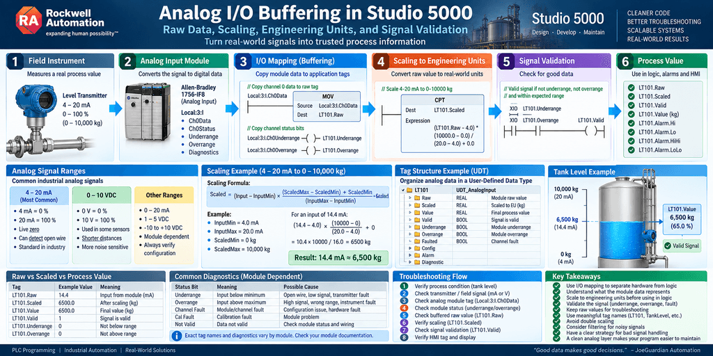
In the previous article, we built a complete digital I/O architecture.

Digital signals are relatively simple:

0 = OFF
1 = ON

Analog signals are different.

An analog input may represent:

• Tank level
• Pressure
• Temperature
• Flow
• Speed
• Weight
• pH
• Conductivity
• Valve position
• Motor current

Instead of asking:

Is the signal ON or OFF?

we must ask:

What value does the signal represent?

And just as important:

Is that value valid?

A robust analog architecture normally needs more than simple I/O mapping.

It may include:

Field Instrument
      ↓
Analog Input Module
      ↓
Module Data
      ↓
Raw / Input Value
      ↓
Scaling
      ↓
Engineering Units
      ↓
Signal Validation
      ↓
Process Value
      ↓
Control Logic / HMI

This is where analog I/O buffering becomes especially valuable.

What Is an Analog Signal?

Unlike a digital signal, an analog signal represents a continuously varying process value.

For example, a pressure transmitter might measure:

0–150 PSI

and communicate that measurement using:

4–20 mA

The relationship is:

4 mA  = 0 PSI
20 mA = 150 PSI

Values between those limits represent intermediate pressures.

For example:

12 mA

is approximately halfway through the signal span.

Therefore:

12 mA ≈ 75 PSI

Common Industrial Analog Signals

Two very common industrial analog signal types are:

4–20 mA

and:

0–10 VDC

Other ranges also exist depending on the instrument and module.

Examples include:

0–20 mA
1–5 V
-10 to +10 V

Always verify the field instrument and I/O module configuration.

Why 4–20 mA Is So Common

The 4–20 mA standard has an important advantage.

The minimum measurement is not:

0 mA

It is:

4 mA

This provides what is often called a:

Live Zero

For example:

4 mA = valid zero measurement

while a signal near:

0 mA

may indicate a problem such as:

• Broken wire
• Loss of transmitter power
• Open circuit
• Device failure

depending on the system design.

This gives 4–20 mA loops useful diagnostic capability.

The Analog Signal Path

Consider a tank level transmitter.

The process path could be:

Tank Level
    ↓
Level Transmitter
    ↓
4–20 mA Signal
    ↓
Analog Input Module
    ↓
PLC Input Data
    ↓
Scaling
    ↓
Tank Level %

The PLC does not directly understand:

The tank contains 63% product.

It receives data from the input module.

That data must be interpreted correctly.

Module Data in Studio 5000

Studio 5000 creates module-defined tags for configured analog modules.

Depending on the specific module and configuration, you may see channel data and diagnostic members such as:

Ch0Data
Ch0Status
Ch0Underrange
Ch0Overrange
Ch0CalFault

The exact member names vary by module and communication format, so you should always verify the specific hardware documentation.

Rockwell analog module definitions can expose per-channel status including underrange, overrange, and calibration-fault indicators.

Example Analog Input

Suppose Channel 0 contains tank level data.

The physical/module value may appear as something similar to:

Local:3:I.Ch0Data

Instead of using this directly throughout the program, we create:

AI_Tank_Level_Raw

or, in a structured design:

TankLevel.Raw

Then:

Local:3:I.Ch0Data
        ↓
AI_Tank_Level_Raw

This separates the physical module from the application logic.

The Analog Buffer Layer

A practical architecture may be:

MODULE DATA
    ↓
RAW BUFFER
    ↓
SCALING
    ↓
VALIDATION
    ↓
PROCESS VALUE

For example:

Local:3:I.Ch0Data
        ↓
AI_Tank_Level.Raw
        ↓
AI_Tank_Level.EU
        ↓
AI_Tank_Level.Valid
        ↓
Process Logic

This gives us multiple troubleshooting points.

Raw Value vs Engineering Units

The raw or unscaled input value is not necessarily the value the operator wants to see.

Suppose the module provides:

4.0

through:

20.0

representing milliamps.

The process range is:

0–100 %

Then we need to convert:

4.0 mA → 0 %
20.0 mA → 100 %

This conversion is called:

Scaling

Rockwell’s current Process Analog Input instruction follows this same concept: an unscaled input range is converted into engineering-unit minimum and maximum values.

The Scaling Equation

The general linear scaling formula is:

Scaled =
(Input - InputMin)
×
(ScaledMax - ScaledMin)
/
(InputMax - InputMin)
+
ScaledMin

This equation works for many linear analog signals.

Example: 4–20 mA to 0–100%

Assume:

InputMin  = 4
InputMax  = 20

ScaledMin = 0
ScaledMax = 100

If the transmitter produces:

12 mA

then:

Scaled =
(12 - 4)
×
(100 - 0)
/
(20 - 4)
+
0

So:

Scaled =
8 × 100 / 16

which gives:

50 %

Example: Pressure Transmitter

Suppose a transmitter is configured:

4–20 mA
=
0–150 PSI

Then:

InputMin  = 4
InputMax  = 20

EUMin     = 0
EUMax     = 150

If the input is:

12 mA

then:

Pressure = 75 PSI

The PLC should ideally work with:

75.0 PSI

rather than requiring every routine to interpret:

12.0 mA

Engineering Units

Engineering Units, often abbreviated:

EU

are the real-world units of the process.

Examples:

PSI
GPM
°C
°F
%
RPM
kg
lb
pH
mS/cm

A good analog architecture converts hardware-oriented data into engineering units as early as practical.

Instead of:

AI_Tank_Pressure_Raw

being used everywhere, application logic should generally work with:

AI_Tank_Pressure_EU

or:

TankPressure.Value

Why Engineering Units Help Troubleshooting

Consider this comparison.

Raw Value

12643

What does that mean?

The technician must know:

• Module type
• Configured range
• Scaling
• Instrument span

Now compare:

TankPressure.Value = 84.3 PSI

The process condition is immediately understandable.

That greatly improves troubleshooting.

Raw Counts

Some analog architectures present values as raw integer counts.

For example, conceptually:

RawMin = 0
RawMax = 32767

or another module-specific range.

Then:

0 → 0 PSI
32767 → 150 PSI

However:

Do not assume a universal raw range for Studio 5000 analog modules.

The representation depends on the specific module, channel configuration, data format, and hardware family.

Always verify the exact module documentation and configuration.

The Module May Already Scale the Signal

Another important point:

Not every Studio 5000 project needs a raw-count scaling equation.

Some analog modules can be configured so that the channel data already represents useful engineering or floating-point values.

For example, depending on module configuration, the controller may receive something close to:

4.0–20.0

or directly scaled engineering values.

Therefore:

Never add scaling blindly.

First determine what the module’s ChxData value actually represents.

Avoid Double Scaling

This is a common problem.

Suppose the analog module is already configured:

4 mA  → 0 PSI
20 mA → 150 PSI

and therefore:

Local:3:I.Ch0Data

already reports:

75 PSI

If the PLC then scales that value again as if it were raw counts, the result will be incorrect.

Before writing scaling logic, always ask:

What exactly does the module data represent?

Studio 5000 vs SLC/RSLogix 500 Thinking

Technicians coming from SLC or MicroLogix systems may remember:

SCP

the Scale with Parameters instruction.

Studio 5000 architectures often handle scaling differently.

Depending on the project, scaling may be performed through:

• Module configuration
• Mathematical instructions
• CPT
• Function blocks
• AOIs
• PlantPAx process instructions
• Custom reusable routines

The concept remains the same:

INPUT RANGE
      ↓
SCALING
      ↓
ENGINEERING RANGE

The implementation may differ.

Scaling With CPT

One approach is to use:

CPT

with the scaling formula.

Conceptually:

CPT
Destination: AI_Pressure_EU

Expression:

((Raw - RawMin) *
(EUMax - EUMin) /
(RawMax - RawMin))
+ EUMin

This makes the calculation explicit.

For training purposes, this is useful because it shows exactly how scaling works.

A Structured Analog Tag

Instead of separate flat tags:

AI_Level_Raw
AI_Level_EU
AI_Level_Hi
AI_Level_HiHi
AI_Level_Lo
AI_Level_LoLo
AI_Level_Bad

we could create:

AI_TankLevel

with members such as:

AI_TankLevel.Raw
AI_TankLevel.Value
AI_TankLevel.Valid
AI_TankLevel.Underrange
AI_TankLevel.Overrange

AI_TankLevel.Alarm.Hi
AI_TankLevel.Alarm.HiHi
AI_TankLevel.Alarm.Lo
AI_TankLevel.Alarm.LoLo

This is a good use case for a UDT.

Example Analog Input UDT

A simplified structure could contain:

UDT_AnalogInput

Raw             REAL
Value           REAL
Valid           BOOL
Underrange      BOOL
Overrange       BOOL
Faulted         BOOL

RawMin          REAL
RawMax          REAL

EUMin           REAL
EUMax           REAL

Then create:

TankPressure

using:

UDT_AnalogInput

Now:

TankPressure.Raw
TankPressure.Value
TankPressure.Valid

all belong to the same instrument.

Signal Validation

Scaling is only half the job.

We also need to determine whether the signal is trustworthy.

Possible problems include:

• Underrange
• Overrange
• Channel fault
• Calibration fault
• Broken wire
• Transmitter fault
• Loss of transmitter power
• Communication failure
• Physically impossible process value

This is why a good analog architecture contains:

Value

and:

Quality / Validity

Underrange and Overrange

Many Rockwell analog modules expose channel status indicating:

Underrange

and:

Overrange

An underrange indicates that the input is below the channel’s minimum detectable signal, while overrange indicates it exceeds the maximum detectable input.

These diagnostic bits should not automatically be ignored.

They can provide valuable troubleshooting information.

Example

Suppose:

Local:3:I.Ch0Underrange = 1

The application might map:

TankPressure.Underrange = 1

Then:

TankPressure.Valid = 0

The HMI can indicate:

PRESSURE SIGNAL BAD

instead of simply displaying:

0 PSI

That distinction matters.

Why 0 PSI May Be Misleading

Suppose the pressure transmitter fails.

If the PLC automatically converts the failed signal into:

0 PSI

the operator may believe:

The process truly has zero pressure.

But the actual situation may be:

The PLC has lost the pressure measurement.

Those are completely different process conditions.

A better architecture separates:

Process Value

from:

Signal Quality

Validity Architecture

For example:

TankPressure.Value = 75.3
TankPressure.Valid = 1

means:

Pressure measurement is valid.

But:

TankPressure.Value = 0.0
TankPressure.Valid = 0

means:

Do not trust the displayed pressure.

The HMI and control logic can react accordingly.

Bad Signal Handling

When a signal becomes invalid, the correct response depends on the process.

Possible strategies include:

• Hold last good value
• Force a predefined fallback
• Stop the controlled equipment
• Generate an alarm
• Inhibit automatic control
• Switch to manual mode
• Continue operating with degraded functionality

There is no universal answer.

This is an engineering and process-safety decision.

Do Not Hide the Raw Signal

Even if the control logic only uses:

TankPressure.Value

the raw signal should remain accessible.

For troubleshooting, it is valuable to see:

TankPressure.Raw

along with:

TankPressure.Value
TankPressure.Valid
TankPressure.Underrange
TankPressure.Overrange

This creates a clear diagnostic chain.

Troubleshooting Example

Suppose the HMI displays:

Tank Level = 0 %

A technician can troubleshoot in layers.

Step 1 — Process

Is the tank actually empty?

Step 2 — Instrument

Does the transmitter display a valid level?

Step 3 — Electrical Signal

Measure the loop current.

For example:

12.4 mA

Step 4 — Module Channel Data

Check:

Local:3:I.Ch0Data

Step 5 — Module Diagnostics

Check:

Underrange
Overrange
Channel Fault

Step 6 — Buffered Raw Value

Check:

TankLevel.Raw

Step 7 — Scaled Value

Check:

TankLevel.Value

Step 8 — HMI Tag

Verify that the HMI references the correct PLC value.

This creates a complete troubleshooting path from the process to the screen.

The Analog Troubleshooting Chain

A simple mental model is:

PROCESS
   ↓
SENSOR
   ↓
TRANSMITTER
   ↓
4–20 mA
   ↓
FIELD WIRING
   ↓
ANALOG MODULE
   ↓
CHANNEL DATA
   ↓
RAW BUFFER
   ↓
SCALING
   ↓
VALIDATION
   ↓
PLC PROCESS VALUE
   ↓
HMI

Whenever the displayed value is incorrect, move through this chain systematically.

Example Tank Level Architecture

Suppose:

LT_101

is a tank level transmitter.

Range:

4–20 mA
=
0–10,000 kg

PLC structure:

LT101.Raw
LT101.Value
LT101.Valid
LT101.Underrange
LT101.Overrange

The flow is:

Level Transmitter
      ↓
4–20 mA
      ↓
Analog Input Channel
      ↓
LT101.Raw
      ↓
Scaling
      ↓
LT101.Value
      ↓
Process Logic

Scaling Example

Suppose:

Input = 14.4 mA

Range:

4–20 mA

Engineering range:

0–10,000 kg

Then:

(14.4 - 4)
/
(20 - 4)
=
0.65

Therefore:

0.65 × 10,000
=
6,500 kg

The PLC should display approximately:

LT101.Value = 6500 kg

High and Low Alarms

Once the signal is in engineering units, alarms become easier to understand.

For example:

TankLevel.Value >= 9000 kg

could generate:

High Alarm

and:

TankLevel.Value >= 9500 kg

could generate:

High-High Alarm

Likewise:

TankLevel.Value <= 1000 kg

might generate:

Low Alarm

Engineering units make alarm setpoints much easier to configure and troubleshoot.

Hi vs HiHi

A typical analog alarm structure may include:

HiHi
Hi
Lo
LoLo

Conceptually:

HIHI     Emergency / critical high condition

HI       High process warning

NORMAL

LO       Low process warning

LOLO     Critical low condition

The actual response depends on the process.

Not every analog signal requires all four alarms.

Analog Alarm Deadband

Another useful consideration is:

Deadband

Suppose the High Alarm is:

90 PSI

Without deadband, a noisy signal moving between:

89.9
90.1
89.8
90.2

could repeatedly activate and clear the alarm.

A deadband might require the value to fall below:

88 PSI

before the alarm clears.

This reduces alarm chatter.

Filtering Analog Signals

Analog signals can also contain noise.

For example:

74.9
75.3
74.8
75.5
75.0

The PLC may use filtering to smooth the measurement.

But:

Filtering and buffering are different concepts.

Buffering transfers or organizes data.

Filtering modifies how rapidly the process value responds to changing input.

Rockwell’s current Process Analog Input functionality, for example, includes both scaling and filtering as separate functions.

Too Much Filtering Can Be Dangerous

Filtering improves stability but adds response delay.

For example:

Real Process Change
       ↓
Heavy Filter
       ↓
Slow PLC Response

Therefore:

Do not add large filters simply to make a noisy signal look smooth.

First determine why the signal is noisy.

Possible causes include:

• Poor grounding
• Shielding problems
• Electrical interference
• Bad transmitter
• Loose connection
• Incorrect routing near VFD cables
• Poor instrument power
• Process turbulence

Filtering should not be used to hide a physical problem.

Analog Input Processing Layers

A strong architecture may use:

Physical Input
      ↓
Raw Buffer
      ↓
Signal Validation
      ↓
Scaling
      ↓
Filtering
      ↓
Engineering Value
      ↓
Alarm Processing
      ↓
Process Logic

The exact order may vary depending on the application.

The important point is that each function has a defined purpose.

Raw vs Scaled vs Process Value

Sometimes three separate values are useful.

Raw

TankLevel.Raw

What the input layer receives.

Scaled

TankLevel.Scaled

Converted to engineering units.

Value

TankLevel.Value

The final value used by the application after validation, substitution, filtering, or simulation.

Conceptually:

Raw
 ↓
Scaled
 ↓
Validated / Filtered
 ↓
Value

This gives excellent visibility during troubleshooting.

Simulation

Analog signals can also benefit from a simulation layer.

For example:

TankLevel.RealValue
TankLevel.SimValue
TankLevel.SimEnable

Then:

If SimEnable = 0
Use RealValue

If SimEnable = 1
Use SimValue

The process logic always uses:

TankLevel.Value

This allows simulation without rewriting the control logic.

Maintenance Substitution

Simulation is not the only reason to substitute an analog value.

During maintenance, there may be legitimate procedures where a known substitute value is used.

For example:

Instrument unavailable
      ↓
Maintenance substitute enabled
      ↓
Known temporary value

This should be controlled carefully and clearly indicated to operators.

Modern process instructions can explicitly support maintenance overrides or substitute PV behavior for this reason.

Analog UDT Example

A more complete analog UDT could look like:

UDT_AnalogInput

Raw             REAL
Scaled          REAL
Value           REAL

Valid           BOOL
Faulted         BOOL
Underrange      BOOL
Overrange       BOOL

SimEnable       BOOL
SimValue        REAL

RawMin          REAL
RawMax          REAL
EUMin           REAL
EUMax           REAL

Alarm.HiHi      BOOL
Alarm.Hi        BOOL
Alarm.Lo        BOOL
Alarm.LoLo      BOOL

Config.HiHiSP   REAL
Config.HiSP     REAL
Config.LoSP     REAL
Config.LoLoSP   REAL

Then:

TankLevel
TankPressure
LinePressure
FlowRate

can all use a similar standardized structure.

But Do Not Build a Giant UDT Automatically

As with the previous article:

Use only the members the application actually needs.

A simple analog transmitter may only require:

Raw
Value
Valid
Faulted

A critical process instrument may justify:

Alarms
Simulation
Maintenance substitution
Rate of change
Filtering
Diagnostics

The architecture should match the process.

Process Analog Input Instructions

In newer Rockwell process-oriented architectures, Rockwell provides process analog functionality that can combine several of these concepts.

For example, Rockwell’s current Process Analog Input instruction can handle functions including:

• Raw-to-engineering scaling
• Filtering
• Input quality
• Out-of-range monitoring
• Maintenance substitution
• Min/max capture
• Rate of change
• Alarms

That illustrates an important point:

Industrial analog processing is usually more than one scaling equation.

Analog I/O Is a Data Quality Problem

Digital signals often ask:

Is it ON?

Analog systems ask:

What is the value?

but they also ask:

Can I trust the value?

That second question is extremely important.

A robust PLC should understand the difference between:

Tank pressure = 0 PSI

and:

Tank pressure measurement unavailable

Those conditions should not automatically be treated as equivalent.

A Complete Architecture

A practical analog input architecture could look like:

┌──────────────────────────────┐
│ Field Transmitter            │
│ 4–20 mA / 0–10 V            │
└─────────────┬────────────────┘
              ↓
┌──────────────────────────────┐
│ Analog Input Module          │
└─────────────┬────────────────┘
              ↓
┌──────────────────────────────┐
│ Module-Defined Channel Data  │
│ Data / Status / Diagnostics  │
└─────────────┬────────────────┘
              ↓
┌──────────────────────────────┐
│ Analog Input Mapping         │
│ Raw + Status                 │
└─────────────┬────────────────┘
              ↓
┌──────────────────────────────┐
│ Scaling                      │
│ Raw → Engineering Units      │
└─────────────┬────────────────┘
              ↓
┌──────────────────────────────┐
│ Validation / Filtering       │
└─────────────┬────────────────┘
              ↓
┌──────────────────────────────┐
│ Process Value                │
│ PSI / % / GPM / °C / kg     │
└─────────────┬────────────────┘
              ↓
┌──────────────────────────────┐
│ Control Logic / HMI / Alarms │
└──────────────────────────────┘

Practical Troubleshooting Example

Suppose:

HMI Tank Weight = 10,000 kg

but the tank is clearly much lighter.

Do not immediately assume the PLC scaling is wrong.

Check the system methodically:

1. Verify actual process condition

2. Check transmitter / load-cell indicator

3. Verify field signal

4. Check analog module channel value

5. Check module status

6. Check buffered raw value

7. Verify scaling parameters

8. Check engineering-unit value

9. Check HMI tag/reference

This approach prevents unnecessary component replacement.

Common Analog Problems

Typical analog troubleshooting issues include:

• Wrong transmitter range
• Wrong PLC scaling
• Wrong analog module range
• 0–20 mA configured instead of 4–20 mA
• Current input vs voltage input mismatch
• Wiring polarity issue
• Broken loop
• Missing loop power
• Ground loop
• Electrical noise
• Bad shield termination
• Module underrange
• Module overrange
• Incorrect engineering-unit limits
• HMI reading the wrong tag
• Double scaling
• Calibration error

A layered analog architecture makes these problems much easier to isolate.

Practical Rules

Rule 1

Know what the module data represents before scaling it.

Rule 2

Do not assume every analog module uses the same raw-count range.

Rule 3

Convert data into engineering units before using it widely in process logic.

Rule 4

Keep the raw value accessible for troubleshooting.

Rule 5

Track signal quality separately from process value.

Rule 6

Do not treat a failed signal automatically as a valid zero measurement.

Rule 7

Use module diagnostic information when available.

Rule 8

Do not confuse buffering, scaling, filtering, and validation.

Rule 9

Avoid double scaling.

Rule 10

Document:

Instrument Range
Signal Range
PLC Range
Engineering Units

Final Thought

Analog I/O buffering is not simply:

MOV Analog_Input Analog_Tag

A robust analog architecture answers several questions:

What did the hardware receive?

What does that number represent?

What are the engineering units?

Is the signal valid?

Is the process value believable?

What should the machine do if the instrument fails?

When those questions are handled explicitly, the PLC becomes much easier to troubleshoot and the process becomes much easier to understand.

The objective is to transform:

Raw Data

into:

Trusted Process Information

That is the real purpose of a good analog input architecture.

Next Article

Analog Output Architecture in Studio 5000 — Setpoints, Limits, Scaling, and Safe Output Commands

In the next article, we will reverse the data flow.

Instead of:

Field Instrument
      ↓
PLC

we will build:

PLC Setpoint
      ↓
Limits / Clamp
      ↓
Engineering Units
      ↓
Scaling
      ↓
Analog Output Buffer
      ↓
Analog Output Module
      ↓
VFD / Control Valve

We will examine:

• 0–100% commands
• 4–20 mA outputs
• 0–10 V outputs
• VFD speed references
• Control valve position
• Min/max limiting
• Clamping
• Manual commands
• Safe fallback values
• Output scaling
• Analog output UDTs
• Troubleshooting from PLC command to field device