10. Building the Complete I/O Layer in Studio 5000 — From Physical Hardware to Industrial Application Logic
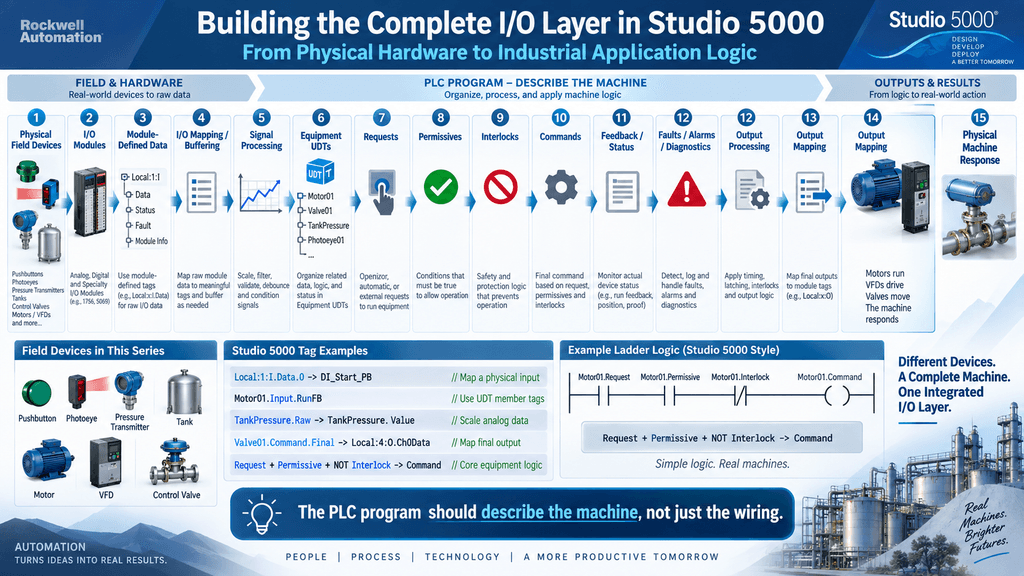
Throughout this series, we have explored several different ways to handle I/O in Studio 5000.
We started with the simplest possible approach:
Local:1:I.Data.0Then we introduced:
Alias Tags
Individual Mapping
MOV
COP
CPS
UDTs
Digital I/O Processing
Analog Scaling
Analog Output Processing
Performance Analysis
Each technique solved a different problem.
Now we can answer the most important question:
How do we combine all of these techniques into one clean industrial PLC architecture?
The answer is not:
Use every technique everywhere.
The answer is:
Build layers, give each layer a clear responsibility, and choose the simplest tool that solves the problem correctly.
The Complete I/O Architecture
A mature Studio 5000 architecture may look like this:
PHYSICAL FIELD DEVICES
        ↓
I/O MODULES
        ↓
MODULE-DEFINED DATA
        ↓
I/O MAPPING / BUFFERING
        ↓
SIGNAL PROCESSING
        ↓
APPLICATION / EQUIPMENT DATA
        ↓
REQUESTS
        ↓
PERMISSIVES
        ↓
INTERLOCKS
        ↓
COMMANDS
        ↓
FEEDBACK / STATUS
        ↓
FAULTS / ALARMS
        ↓
OUTPUT PROCESSING
        ↓
OUTPUT MAPPING
        ↓
PHYSICAL FIELD DEVICES
This is not simply an I/O strategy.
It is a complete data-flow architecture.
Layer 1 — Physical Field Devices
Everything begins in the real machine.
Examples include:
Pushbuttons
Photoeyes
Limit Switches
Proximity Sensors
Pressure Switches
Motor Overloads
VFD Status
Transmitters
Control Valves
Motor Starters
Solenoids
These devices exist independently of the PLC program.
The first question during troubleshooting should often be:
What is physically happening?
not:
What does the ladder say?
Layer 2 — I/O Modules
The field devices connect to physical or networked I/O.
For example:
Digital Input Module
Digital Output Module
Analog Input Module
Analog Output Module
Remote I/O Adapter
VFD Ethernet Connection
When supported modules are added to a Studio 5000 project, Logix Designer creates corresponding module-defined tags.
Examples may look like:
Local:1:I
Local:1:O
Local:1:C
or structured device tags containing members such as:
Ready
Active
Faulted
Data
depending on the device.
This is the hardware-facing layer of the controller.
Layer 3 — Module-Defined Data
This is an important concept.
The module-defined tag represents the controller’s interface to the configured hardware.
For example:
Local:1:I.Data.0might represent:
Start Pushbuttonor a networked drive may expose:
Drive:I.Ready
Drive:I.Active
Drive:I.Faulted
These tags are valid and important.
But the question is:
Should application logic use them everywhere?
Sometimes yes.
Often, especially in larger projects, no.
Layer 4 — I/O Mapping / Buffering
This layer creates the boundary between:
Hardwareand:
Application LogicFor a digital input:
Local:1:I.Data.0
        ↓
DI_Start_PB
For a motor structure:
Local:1:I.Data.2
        ↓
Motor01.Input.RunFB
For an analog channel:
Local:3:I.Ch0Data
        ↓
TankPressure.Raw
This is where several methods from this series may be used.
Which Mapping Method Belongs Here?
Not every signal needs the same method.
For individual Boolean signals:
XIC / XIO → OTEmay be clear and easy to troubleshoot.
For individual numeric values:
MOVmay be appropriate.
For a normal contiguous block:
COPmay be appropriate.
For a data set that requires a coherent snapshot:
CPSmay be appropriate.
For small systems:
Alias Tagsmay provide all the abstraction required.
The mapping method should match the type of data.
A Hybrid Architecture Is Normal
A good Studio 5000 project might use all of these:
Aliasfor a few simple physical signals,
XIC / OTEfor discrete field mapping,
MOVfor analog values,
CPSfor a network data snapshot,
and:
UDTsfor equipment organization.
That is not inconsistent.
It is good engineering when each method has a purpose.
Layer 5 — Signal Processing
The mapped input is not always ready for control logic.
Some signals require additional processing.
For digital inputs:
Debounce
Filtering
Inversion
Validation
Contradictory Sensor Detection
For analog inputs:
Scaling
Filtering
Range Checking
Signal Validation
Simulation
Conceptually:
RAW SIGNAL
    ↓
PROCESSING
    ↓
TRUSTED APPLICATION SIGNAL
Example Digital Signal
Suppose:
Local:1:I.Data.0is a mechanical Start Pushbutton.
Input mapping:
Local:1:I.Data.0
        ↓
DI_Start_PB_Raw
Debounce:
DI_Start_PB_Raw
        ↓
100 ms stable
        ↓
DI_Start_PB
The request logic uses:
DI_Start_PBnot necessarily the raw electrical signal.
Example Normally Closed Signal
Suppose:
Local:1:I.Data.3represents a healthy motor overload circuit.
Map it as:
Motor01.Input.OL_OKwhere:
1 = Healthy
0 = Not Healthy
Then the rest of the program does not need to repeatedly interpret the wiring philosophy.
This keeps electrical meaning near the I/O layer.
Example Analog Signal
Suppose a pressure transmitter produces:
4–20 mArepresenting:
0–150 PSIThe architecture may be:
Analog Module
      ↓
TankPressure.Raw
      ↓
Scaling
      ↓
TankPressure.Scaled
      ↓
Validation
      ↓
TankPressure.Value
The control logic uses:
TankPressure.Valuein PSI.
The raw signal remains available for troubleshooting.
Layer 6 — Application / Equipment Data
Once signals are mapped and processed, we enter the application layer.
This is where UDTs become extremely useful.
Instead of:
Motor1_FB
Motor1_OL
Motor1_Run
Motor1_Fault
we can organize:
Motor01.Input.RunFB
Motor01.Input.OL_OK

Motor01.Request.Start

Motor01.Permissive.Run

Motor01.Command.Run

Motor01.Status.Running

Motor01.Fault.StartFail
The PLC program begins to resemble the equipment it controls.
UDTs Organize Data
Remember:
UDT = Data StructureA UDT does not automatically:
- Buffer I/O
- Control a motor
- Detect faults
- Provide safety
It organizes related data.
For repetitive equipment, that is extremely valuable.
Rockwell’s Data Type Editor also exposes the actual size of user-defined structures in bytes, which reinforces that UDTs are real controller data structures rather than merely cosmetic folders.
Layer 7 — Requests
A physical input should not necessarily become a physical output directly.
For example:
Start Pushbuttonshould typically create:
Motor01.Request.Startrather than:
Motor Output = ONRequests represent:
What someone or something wants the machine to do.
Sources may include:
Operator
HMI
Automatic Sequence
SCADA
Recipe
State Machine
Another Equipment Module
Example
DI_Start_PB
      ↓
Motor01.Request.Start
The request alone does not guarantee that the motor will run.
The PLC still needs to determine whether operation is allowed.
Layer 8 — Permissives
Permissives answer:
Are the required conditions available to start or continue operation?
Examples:
Safety OK
Overload OK
VFD Ready
Air Pressure OK
Correct Mode
No Critical Fault
Upstream Equipment Ready
For example:
Motor01.Permissive.Runmight require:
Motor01.Input.OL_OK
AND
Safety_OK
AND
Drive01.Status.Ready
Permissive vs Request
This distinction is important.
Requestmeans:
Run the motor.
Permissivemeans:
Conditions allow the motor to run.
Neither alone should necessarily energize the output.
Layer 9 — Interlocks
Interlocks answer:
Is there an active condition that must prevent or stop operation?
Examples:
Downstream Conveyor Stopped
Tank High-High
Valve Not Open
Guard Open
Process Condition Invalid
A useful conceptual relationship is:
Request
AND
Permissive
AND
NOT Interlocked
      ↓
Command
Permissive vs Interlock
A simple way to think about them:
Permissive = What must be true
Interlock  = What must not be active
Different facilities may use different naming philosophies.
Consistency matters more than terminology.
Layer 10 — Commands
The command represents:
What the PLC has finally decided the equipment should do.
For example:
Motor01.Command.RunThis should be different from:
Motor01.Request.Startbecause the PLC may receive a request but reject it because of:
Missing Permissive
Interlock
Fault
Wrong Mode
That distinction dramatically improves troubleshooting.
Example
Suppose:
Motor01.Request.Start = 1but:
Motor01.Permissive.Run = 0Then:
Motor01.Command.Run = 0A technician can immediately see:
The request exists, but the PLC is not allowing the command.
That is much easier to troubleshoot than one giant rung.
Layer 11 — Feedback and Status
Commands represent what the PLC wants.
Feedback represents what the machine actually reports.
For example:
Motor01.Command.Run = 1does not mean:
Motor01.Status.Running = 1until actual feedback confirms it.
This is fundamental.
Command vs Feedback
Command = PLC intention

Feedback = field response

Status = interpreted machine condition
For example:
Motor01.Command.Run = 1

Motor01.Input.RunFB = 1

Motor01.Status.Running = 1
That is a healthy sequence.
Failure Example
Suppose:
Motor01.Command.Run = 1but:
Motor01.Input.RunFB = 0after five seconds.
The PLC may generate:
Motor01.Fault.StartFail = 1This is where clean I/O architecture becomes powerful diagnostics.
Layer 12 — Faults
Faults represent abnormal equipment conditions that typically require corrective action.
Examples:
Motor Start Failure
Motor Overload
Valve Travel Failure
Sensor Contradiction
Analog Signal Invalid
VFD Fault
Communication Failure
Fault logic should generally use meaningful application signals rather than raw hardware addresses.
For example:
Motor01.Command.Run
AND
NOT Motor01.Input.RunFB
AND
StartTimer.DN
      ↓
Motor01.Fault.StartFail
That logic reads almost like a troubleshooting statement.
Layer 13 — Alarms
Faults and alarms are related but not necessarily identical.
A fault may represent:
Equipment Abnormal Conditionwhile an alarm represents:
Condition that should be presented to an operatorFor example:
Motor01.Fault.StartFailmay drive:
Motor01.Alarm.StartFailwhich is then displayed on the HMI.
Some systems combine these concepts.
Others keep them separate.
Again, consistency is key.
Layer 14 — Diagnostics
Good industrial programs expose enough information to explain:
Why isn’t the equipment working?
Diagnostics might include:
Missing Permissive
Active Interlock
Start Timer
Stop Timer
Command / Feedback Difference
Analog Signal Quality
Communication Status
Simulation Active
Maintenance Override
The goal is not to generate hundreds of diagnostic bits.
The goal is to expose the information technicians actually need.
Layer 15 — Output Processing
Outputs should not always go directly from command to hardware.
Digital outputs may require:
Final Ownership
Mode Handling
Simulation Selection
Analog outputs may require:
Command Source Selection
Limits
Clamp
Interlock Safe Value
Ramp
Scaling
For example:
Valve01.Command.Requested = 80 %but:
Valve01.Config.Max = 70 %so:
Valve01.Command.Final = 70 %The output architecture preserves both values for troubleshooting.
Layer 16 — Output Mapping
Now the final application command reaches the physical hardware.
For a digital output:
Motor01.Command.Run
        ↓
Local:2:O.Data.0
For an analog output:
Valve01.Command.Final
        ↓
Local:4:O.Ch0Data
assuming the data representation matches the configured module.
Only here does the application reconnect to the physical output.
One Final Owner Per Output
One of the strongest architecture rules in this entire series is:
Each physical output should have one clearly defined final software owner.
Avoid:
Routine A writes Local:2:O.Data.0
Routine B writes Local:2:O.Data.0
Routine C writes Local:2:O.Data.0
Prefer:
Many logical conditions
        ↓
Motor01.Command.Run
        ↓
ONE Output Mapping Rung
        ↓
Local:2:O.Data.0
That makes troubleshooting dramatically easier.
Complete Digital Motor Example
Let’s combine everything.
Physical I/O:
Local:1:I.Data.0    Start PB
Local:1:I.Data.1    Stop OK
Local:1:I.Data.2    Motor FB
Local:1:I.Data.3    Overload OK

Local:2:O.Data.0    Motor Starter
Application structure:
Motor01.Input.StartPB
Motor01.Input.StopOK
Motor01.Input.RunFB
Motor01.Input.OL_OK

Motor01.Request.Start

Motor01.Permissive.Run

Motor01.Interlock.Active

Motor01.Command.Run

Motor01.Status.Running

Motor01.Fault.StartFail
Motor01.Fault.Overload
Step 1 — Input Mapping
Local:1:I.Data.0
        ↓
Motor01.Input.StartPB
Local:1:I.Data.1
↓
Motor01.Input.StopOKLocal:1:I.Data.2
↓
Motor01.Input.RunFBLocal:1:I.Data.3
↓
Motor01.Input.OL_OKStep 2 — Request
Motor01.Input.StartPB
↓
Motor01.Request.StartStep 3 — Permissive
Motor01.Input.StopOK
AND
Motor01.Input.OL_OK
AND
Safety_OK
↓
Motor01.Permissive.RunStep 4 — Interlock
Example:
Downstream_Faulted
↓
Motor01.Interlock.ActiveStep 5 — Command
Motor01.Request.Start
AND
Motor01.Permissive.Run
AND
NOT Motor01.Interlock.Active
↓
Motor01.Command.RunStep 6 — Output Mapping
Motor01.Command.Run
↓
Local:2:O.Data.0Step 7 — Feedback
The motor runs.
Auxiliary feedback returns:
Local:1:I.Data.2
        ↓
Motor01.Input.RunFBStep 8 — Status
Motor01.Command.Run
AND
Motor01.Input.RunFB
      ↓
Motor01.Status.Running
Step 9 — Fault
If:
Command.Run = 1
RunFB = 0
StartTimer.DN = 1
then:
Motor01.Fault.StartFail = 1Now the entire equipment chain is visible.
Complete Analog Input Example
Suppose:
PT101is a pressure transmitter.
Range:
4–20 mA
0–150 PSI
Architecture:
PT101 Transmitter
       ↓
Analog Input Module
       ↓
Module Channel Data
       ↓
PT101.Raw
       ↓
Scaling
       ↓
PT101.Scaled
       ↓
Validation
       ↓
PT101.Value
       ↓
Process Logic / HMI
Application structure:
PT101.Raw
PT101.Scaled
PT101.Value

PT101.Valid
PT101.Underrange
PT101.Overrange

PT101.Alarm.Hi
PT101.Alarm.HiHi
Complete Analog Output Example
Suppose:
FCV101is a flow-control valve.
Architecture:
PID Output
      ↓
FCV101.Command.Requested
      ↓
Limits
      ↓
Interlock
      ↓
Ramp
      ↓
FCV101.Command.Final
      ↓
Analog Output Mapping
      ↓
Analog Module
      ↓
4–20 mA
      ↓
Valve Positioner
Now troubleshooting can compare:
Requested
Limited
Final
Physical Output
Field Feedback
at every stage.
Where Alias Tags Fit
Alias Tags are still useful.
They are excellent when you want:
Meaningful Nameswithout creating an independent buffer.
For a small machine:
DI_Start_PB
Alias For Local:1:I.Data.0
may be completely adequate.
Do not reject Alias Tags simply because a more complex architecture exists.
Where Individual Mapping Fits
Individual mapping is excellent when:
Each physical signal should be easy to trace.For example:
Local:1:I.Data.4
        ↓
DI_Photoeye
The technician can monitor both sides of the rung.
This is one reason individual mapping remains attractive in many industrial machines.
Where MOV Fits
MOV works well for individual numeric transfers.
For example:
MOV
Source: Local:3:I.Ch0Data
Dest: PT101.Raw
Simple.
Clear.
Easy to troubleshoot.
Where COP Fits
COP works well when:
A contiguous block of data needs to be copiedand synchronization is not required.
Examples:
Recipes
Arrays
Structures
Backup Data
But remember:
One COP instruction may move a large amount of memory.
Do not judge performance by instruction count alone.
Where CPS Fits
CPS belongs where data consistency matters.
For example:
I/O Snapshot
Produced Data
Consumed Data Processing
Data Modified By Another Task
The concept is:
Live Data
    ↓
CPS
    ↓
Coherent Snapshot
Do not use CPS simply because it appears more robust.
Synchronization should solve a real requirement.
Where UDTs Fit
UDTs belong at the application/equipment layer.
Examples:
Motor01
Valve01
VFD01
Tank01
PT101
Conveyor01
They organize related information.
For repetitive equipment, this creates highly scalable architecture.
Where AOIs Fit
AOIs add reusable behavior.
Remember:
UDT = Data
AOI = Logic
A standardized motor could become:
Motor01
    ↓
AOI_Motor
The AOI processes:
Requests
Permissives
Feedback
Timers
Faults
Status
while the UDT organizes the associated data.
This can be extremely powerful.
But not every small project needs AOIs.
The Architecture Should Grow With the Machine
A simple machine might use:
Alias Tags
+
Basic Logic
A medium machine might use:
Individual Mapping
+
Structured Routines
+
Controller Tags
A larger machine might use:
Mapping
+
UDTs
+
AOIs
+
State Machines
+
Diagnostics
A plant-wide architecture might additionally include:
ISA-88
Equipment Modules
Produced / Consumed Data
Standard HMI Faceplates
Historian Integration
SCADA
Architecture should scale with complexity.
Example Routine Structure
A practical project might use:
MainRoutine

R00_System
R01_Input_Mapping
R02_Input_Processing
R03_Mode_Control
R04_Requests
R05_Permissives
R06_Interlocks
R07_Equipment_Control
R08_Feedback_Status
R09_Fault_Logic
R10_Alarm_Logic
R11_Analog_Processing
R12_Simulation
R13_HMI_Status
R14_Output_Processing
R15_Output_Mapping
Not every project needs all of these.
The important principle is:
Every routine should have a clear responsibility.
Data Flow Matters More Than Routine Numbers
The architecture should visually flow:
INPUT
  ↓
PROCESS
  ↓
DECIDE
  ↓
COMMAND
  ↓
VERIFY
  ↓
DIAGNOSE
  ↓
OUTPUT
Routine names and numbers can vary.
Data flow should remain understandable.
Simulation Layer
A well-designed I/O abstraction layer makes simulation much easier.
For example:
Real Motor Feedback ──┐
                      ├──→ Motor01.Input.RunFB
Simulated Feedback ───┘
selected by:
Simulation_ModeThe application logic remains unchanged.
That is a major advantage.
But Simulation Must Be Explicit
Useful simulation tags might include:
Simulation.Active
Simulation.Permitted
Simulation.OutputBlocked
Simulation.Alarm
A production machine should never accidentally operate on simulated inputs without clear indication.
Simulation is a testing tool, not a hidden bypass.
HMI Integration
The same architecture helps the HMI.
Instead of browsing:
Local:1:I.Data.2
Local:2:O.Data.0
TemporaryBit23
the HMI can work with:
Motor01.Command.Run
Motor01.Status.Running
Motor01.Status.Faulted
Motor01.Fault.StartFail
Now HMI objects and PLC equipment structures speak the same language.
HMI Should Not Become the Control Layer
A good architecture normally keeps core machine control in the PLC.
The HMI should primarily provide:
Commands
Setpoints
Mode Requests
Status
Diagnostics
Alarm Interaction
The PLC should decide whether those requests are safe and valid.
For example:
HMI_Start_Request
        ↓
PLC Permissive / Interlock Logic
        ↓
Motor Command
not:
HMI Button
        ↓
Physical Output
Hardware Changes Become Easier
Suppose:
Motor01.Input.RunFBoriginally maps to:
Local:1:I.Data.3The hardware changes.
Now it comes from:
Remote_IO:4:I.Data.7The application logic can remain:
Motor01.Input.RunFBOnly the I/O mapping layer changes.
That is true hardware abstraction.
Why This Matters During Plant Modernization
Industrial plants frequently experience:
I/O Card Replacement
Rack Changes
Remote I/O Migration
PLC Upgrades
VFD Replacement
Network Migration
A well-defined hardware interface can make these changes less disruptive.
The application logic should describe:
What the machine doesnot:
Where every wire physically landsexcept where that information belongs.
But Never Hide the Hardware Completely
Abstraction should not make troubleshooting harder.
A technician should still be able to answer:
Where does Motor01.RunFB physically come from?
The mapping routine should show:
Local:1:I.Data.3
        ↓
Motor01.Input.RunFB
This is why a visible hardware/application boundary is so useful.
Performance Layer
As discussed in Post 9:
Do not optimize the architecture by guessing.
Monitor:
Task Scan Time
Maximum Scan
Task Period
Overlap Count
If the controller has plenty of margin, maintainability may matter much more than eliminating a few mapping instructions.
If the controller is near its timing limits, measure and optimize the real bottleneck.
Fast and Slow Tasks
Not every signal needs the same update rate.
For example:
High-Speed Registrationmay need a fast periodic task.
But:
Tank Temperaturemay not.
A good architecture may use:
FAST TASK

Critical time-sensitive logic
and:
NORMAL TASK

Machine sequencing
and:
SLOW TASK

Diagnostics
Statistics
HMI support
This often improves performance more meaningfully than removing readable mapping logic.
Naming Standards
A complete architecture needs a naming standard.
One possible convention is:
DI_  Digital Input
DO_  Digital Output
AI_  Analog Input
AO_  Analog Output
For structured equipment:
.Input
.Request
.Permissive
.Interlock
.Command
.Status
.Fault
.Alarm
.Config
.Diagnostic
The exact words are less important than consistency.
Example
Motor01.Input.RunFB
Motor01.Request.Start
Motor01.Permissive.Run
Motor01.Interlock.Active
Motor01.Command.Run
Motor01.Status.Running
Motor01.Fault.StartFail
Motor01.Alarm.StartFail
Without opening the logic, the tag names already tell a story.
Documentation Matters
Rung comments should explain intent.
Weak comment:
Motor RunBetter comment:
Generate the final Motor01 run command when a start request is active,
all run permissives are satisfied, and no active interlock prevents operation.
Good documentation reduces troubleshooting time.
Do Not Comment the Obvious
Avoid comments such as:
If input is on, turn output on.Instead explain:
Why the rung existsand:
What process requirement it implementsThe ladder already shows the Boolean relationship.
The comment should provide engineering context.
A Technician’s Troubleshooting Path
A complete architecture should let a technician follow:
FIELD
 ↓
PHYSICAL INPUT
 ↓
MAPPED INPUT
 ↓
PROCESSED SIGNAL
 ↓
REQUEST
 ↓
PERMISSIVE
 ↓
INTERLOCK
 ↓
COMMAND
 ↓
OUTPUT
 ↓
FIELD DEVICE
 ↓
FEEDBACK
 ↓
STATUS
 ↓
FAULT / ALARM
If that path is easy to follow, the program is doing more than controlling the machine.
It is helping maintain the machine.
Example: Conveyor Will Not Start
Check:
1. DI_Start_PB

2. Conveyor01.Request.Start

3. Conveyor01.Permissive.Run

4. Conveyor01.Interlock.Active

5. Conveyor01.Command.Run

6. Physical Output

7. Motor Feedback

8. StartFail Fault
This provides a systematic troubleshooting process instead of random searching through ladder logic.
Example: Tank Level Looks Wrong
Check:
1. Actual Process

2. Transmitter

3. 4–20 mA Signal

4. Module Channel Data

5. TankLevel.Raw

6. TankLevel.Scaled

7. TankLevel.Valid

8. TankLevel.Value

9. HMI Tag
Same architecture.
Different signal type.
Example: Valve Will Not Open
Check:
1. Requested Position

2. Command Source

3. Min / Max Limits

4. Interlock

5. Final Command

6. Analog Output Tag

7. Physical mA Signal

8. Positioner

9. Valve Feedback
Again, the architecture itself becomes the troubleshooting procedure.
What Not to Do
A difficult PLC architecture often looks like:
Physical Input
      ↓
Random Internal Bit
      ↓
Another Temporary Bit
      ↓
HMI Bit
      ↓
Latch
      ↓
Output
with:
Multiple Writers
No Clear Ownership
No Comments
Physical Addresses Everywhere
The machine may run.
But maintaining it becomes difficult.
Avoid Architecture for Architecture’s Sake
The opposite mistake is also possible.
Do not turn:
One Pushbutton
One Motor
into:
8 UDTs
4 AOIs
12 Routines
3 CPS Buffers
Nested State Machines
simply because advanced tools exist.
Good architecture is proportional.
The Simplest Correct Architecture
A useful engineering principle is:
Use the simplest architecture that remains clear, maintainable, scalable enough, and technically correct for the application.
For one machine that may be:
Alias TagsFor another:
Individual MappingFor another:
UDT + AOIThere is no universal template.
Practical Decision Guide
| Requirement | Good Starting Point |
|---|---|
| Tiny training project | Direct I/O |
| Small readable machine | Alias Tags |
| Industrial machine with troubleshooting focus | Individual Mapping |
| Individual numeric value | MOV |
| Large normal data block | COP |
| Coherent asynchronous dataset | CPS |
| Repetitive equipment | UDT |
| Reusable equipment logic | UDT + AOI |
| Analog transmitter | Mapping + Scaling + Validation |
| Analog actuator | Command Processing + Mapping |
| High-speed application | Measure task performance |
This is a guide, not an absolute rule.
The Architecture We Built Across This Series
We started here:
Local:1:I.Data.0Then learned:
Alias TagsThen:
Mapped TagsThen:
XIC / XIO / OTEThen:
MOVThen:
COP / CPSThen:
UDTsThen:
Digital I/O ProcessingThen:
Analog Input ProcessingThen:
Analog Output ProcessingThen:
Performance MeasurementNow we can see that these are not competing techniques.
They are tools inside one architecture.
The Final Model
A strong Studio 5000 architecture can be summarized as:
┌───────────────────────────────┐
│ PHYSICAL MACHINE              │
└───────────────┬───────────────┘
                ↓
┌───────────────────────────────┐
│ MODULE-DEFINED I/O            │
└───────────────┬───────────────┘
                ↓
┌───────────────────────────────┐
│ I/O MAPPING / BUFFERING       │
│ Alias / XIC-OTE / MOV         │
│ COP / CPS when appropriate    │
└───────────────┬───────────────┘
                ↓
┌───────────────────────────────┐
│ SIGNAL PROCESSING             │
│ Debounce / Scaling / Validate │
└───────────────┬───────────────┘
                ↓
┌───────────────────────────────┐
│ APPLICATION / EQUIPMENT UDTs  │
└───────────────┬───────────────┘
                ↓
┌───────────────────────────────┐
│ REQUESTS                      │
└───────────────┬───────────────┘
                ↓
┌───────────────────────────────┐
│ PERMISSIVES                   │
└───────────────┬───────────────┘
                ↓
┌───────────────────────────────┐
│ INTERLOCKS                    │
└───────────────┬───────────────┘
                ↓
┌───────────────────────────────┐
│ COMMANDS                      │
└───────────────┬───────────────┘
                ↓
┌───────────────────────────────┐
│ FEEDBACK / STATUS             │
└───────────────┬───────────────┘
                ↓
┌───────────────────────────────┐
│ FAULTS / ALARMS / DIAGNOSTICS │
└───────────────┬───────────────┘
                ↓
┌───────────────────────────────┐
│ OUTPUT PROCESSING             │
└───────────────┬───────────────┘
                ↓
┌───────────────────────────────┐
│ OUTPUT MAPPING                │
└───────────────┬───────────────┘
                ↓
┌───────────────────────────────┐
│ PHYSICAL MACHINE              │
└───────────────────────────────┘
This creates a complete circle:
FIELD
  ↓
PLC
  ↓
DECISION
  ↓
FIELD
  ↓
FEEDBACK
  ↓
PLC
Final Rules From the Entire Series
1. Do not confuse Alias Tags with buffering.
An Alias changes how data is referenced.
A buffer creates an independent application representation.
2. Do not use one mapping method everywhere.
Choose the method based on the data and application.
3. Separate hardware from application logic when the project benefits from it.
4. Keep physical I/O easy to trace.
Abstraction should improve troubleshooting, not hide the machine.
5. Separate commands from feedback.
Command ≠ Feedback6. Separate requests from commands.
Request ≠ Permission to operate7. Separate raw analog values from trusted process values.
Raw ≠ Valid Process Information8. Give each output one final owner.
9. Use UDTs to organize related equipment data.
10. Use AOIs for reusable behavior when appropriate.
11. Use COP for normal block copies.
12. Use CPS when synchronization is actually required.
13. Do not confuse buffering, filtering, debounce, scaling, or validation.
They solve different problems.
14. Measure performance instead of guessing.
15. Optimize for the machine—not for a programming benchmark.
Final Thought
The purpose of I/O architecture is not to make a PLC program look sophisticated.
It is to make the relationship between:
FIELD HARDWAREand:
CONTROL SOFTWAREclear and intentional.
A good architecture lets an Automation Technician answer:
What signal entered the PLC?
What does that signal mean?
Is the value valid?
What does the machine want to do?
Are the required conditions satisfied?
What is blocking operation?
What command did the PLC issue?
Did the physical device respond?
If not, why?
When a PLC program can answer those questions clearly, it becomes more than control logic.
It becomes a troubleshooting tool.
That is the real value of industrial I/O architecture.
Series Conclusion
Throughout this series we moved from:
Local:1:I.Data.0to a complete architecture:
Physical I/O
      ↓
Mapping
      ↓
Processing
      ↓
Structured Equipment Data
      ↓
Requests
      ↓
Permissives
      ↓
Interlocks
      ↓
Commands
      ↓
Feedback
      ↓
Diagnostics
      ↓
Physical Outputs
There is no single perfect I/O mapping method.
The best architecture is the one that balances:
Correctness
Safety
Readability
Troubleshooting
Maintainability
Scalability
Performance
for the actual machine.
The goal is not:
Write the most advanced PLC code.
The goal is:
Build control software that another technician can understand, troubleshoot, modify, and trust years later.
That is industrial PLC programming.