JoeGuardian Automation

Bonus — PLC Input and Output Buffering: Building Cleaner and Safer Logic

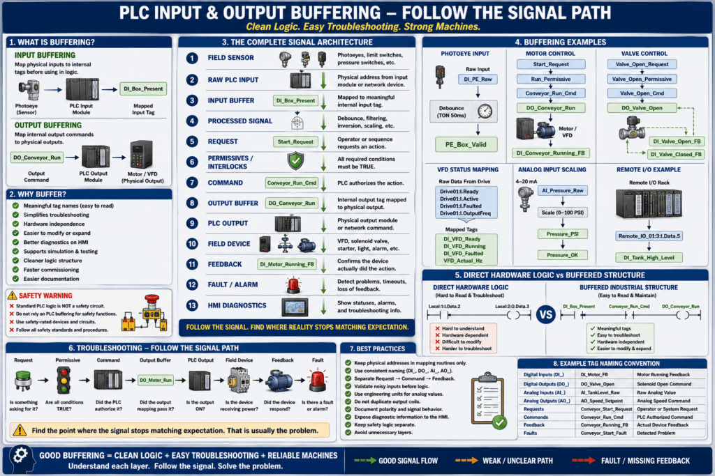
Throughout this PLC series, we repeatedly used an important programming concept:

Do not build your entire machine logic directly from physical I/O addresses.

Instead, create a clean separation between the real hardware and the control logic.

A good signal path looks like this:

Physical Input
      ↓
Input Buffer
      ↓
Internal Logic
      ↓
Command
      ↓
Output Buffer
      ↓
Physical Output
      ↓
Field Device
      ↓
Feedback

This technique is commonly called:

• Input Mapping
• Output Mapping
• I/O Buffering
• I/O Mapping
• Input/Output Abstraction

The terminology may vary, but the idea is the same.

For an automation technician, buffering makes a PLC program easier to:

• Read
• Troubleshoot
• Modify
• Commission
• Document
• Expand

This bonus post brings together many concepts covered throughout the series.

1. What Is PLC Input Buffering?

Input buffering means copying or mapping a physical PLC input into an internal tag before using it in the machine logic.

Instead of using:

Local:1:I.Data.0

everywhere in the program, create a meaningful tag such as:

DI_Box_Present

The mapping becomes:

Local:1:I.Data.0
        ↓
DI_Box_Present

Your machine logic then uses:

DI_Box_Present

instead of the hardware address.

2. What Is PLC Output Buffering?

Output buffering works in the opposite direction.

Instead of controlling:

Local:2:O.Data.3

directly throughout the program, create an internal output command.

Example:

DO_Conveyor_Run

Then map:

DO_Conveyor_Run
       ↓
Local:2:O.Data.3

The machine logic generates:

Conveyor_Run_Cmd

and the output mapping decides what physical output should be energized.

A complete structure could be:

Conveyor_Run_Cmd
       ↓
DO_Conveyor_Run
       ↓
Local:2:O.Data.3
       ↓
Motor Starter / VFD
       ↓
Motor

3. Why Not Use Physical I/O Everywhere?

Consider this rung:

XIC Local:1:I.Data.4
XIC Local:1:I.Data.7
XIO Local:1:I.Data.10
OTE Local:2:O.Data.3

Technically, it may work.

But what does it mean?

Without comments or drawings, you may not know.

Compare it to:

XIC DI_Box_Present
XIC DI_Guard_OK
XIO Conveyor_Fault
OTE Conveyor_Run_Cmd

The second version is immediately easier to understand.

This is one of the biggest benefits of buffering:

The PLC program describes the machine, not the wiring diagram.

4. The Recommended Signal Architecture

A clean industrial PLC design can follow this path:

RAW FIELD SIGNALS
        ↓
INPUT BUFFERING
        ↓
CONDITIONED INPUTS
        ↓
REQUESTS
        ↓
PERMISSIVES / INTERLOCKS
        ↓
COMMANDS
        ↓
OUTPUT BUFFERING
        ↓
PHYSICAL OUTPUTS
        ↓
FIELD DEVICES
        ↓
FEEDBACK
        ↓
FAULTS / ALARMS

This architecture creates a clear separation between:

Hardware
Logic
Commands
Outputs
Feedback
Diagnostics

That separation is extremely useful during troubleshooting.

5. Simple Input Buffering Example

Suppose a photoelectric sensor is connected to:

Local:1:I.Data.2

Instead of using that hardware address throughout the program, create:

DI_PE_Box_Present

Input mapping:

| Local:1:I.Data.2 |----------------( DI_PE_Box_Present )

Now all machine logic uses:

DI_PE_Box_Present

For example:

DI_PE_Box_Present
        ↓
Box_Present
        ↓
Sequence transition

6. Why Use DI_ and DO_ Prefixes?

One useful naming convention is:

DI_ = Digital Input
DO_ = Digital Output
AI_ = Analog Input
AO_ = Analog Output

Examples:

DI_PE_Box_Present
DI_Motor_Running_FB
DI_Motor_Overload
DI_Guard_OK

DO_Conveyor_Run
DO_Valve_Open
DO_Alarm_Horn
DO_Green_Light

The prefix immediately tells the technician what type of signal they are looking at.

7. Raw Input vs Processed Input

Sometimes the mapped input should not be used directly.

You may need another layer.

Example:

Physical Input
      ↓
DI_PE_Box_Raw
      ↓
Debounce Logic
      ↓
PE_Box_Valid

Why?

Because real-world signals can:

Bounce
Flicker
Chatter
Contain electrical noise
Change briefly during motion

The raw input represents what the hardware sees.

The processed tag represents what the program trusts.

8. Example — Photoeye Debounce

Suppose a photoeye flickers when a box enters the detection area.

Raw signal:

DI_PE_Box_Raw

After a short validation timer:

PE_Box_Valid

The signal path becomes:

Photoeye
   ↓
PLC Input
   ↓
DI_PE_Box_Raw
   ↓
Debounce Timer
   ↓
PE_Box_Valid
   ↓
Machine Logic

This makes it easier to diagnose whether a problem is:

Sensor
Wiring
Raw input
Debounce timing
Machine logic

9. Invert Signals in the Mapping Layer

Another useful technique is handling signal polarity during input mapping.

Suppose a device is wired fail-safe and its electrical behavior is:

Input ON  = Healthy
Input OFF = Fault

You may create:

DI_Guard_OK

so that the rest of the program works logically with:

TRUE = Guard Healthy
FALSE = Guard Problem

This is often easier to understand than forcing every routine to remember the original wiring polarity.

10. Example — Normally Closed Field Device

Imagine a normally closed field contact.

Raw hardware input:

Local:1:I.Data.6

If the design is:

1 = Healthy
0 = Fault

you can map:

Local:1:I.Data.6
       ↓
DI_Air_Pressure_OK

Now the program reads naturally:

XIC DI_Air_Pressure_OK

instead of forcing the programmer to interpret the electrical design every time.

11. Keep Physical Inputs Out of Machine Logic

One useful programming rule is:

Physical input addresses should normally appear only in the input mapping section.

Instead of:

Local:1:I.Data.0

appearing in:

Sequence
Motor Control
Valve Logic
Alarms
HMI
Faults

it appears once:

INPUT_MAPPING

and the rest of the program uses:

DI_Box_Present

This creates a single point of reference.

12. Why This Helps When Hardware Changes

Suppose:

Box_Present

was originally wired to:

Local:1:I.Data.2

but maintenance moves the sensor to:

Local:1:I.Data.5

Without input buffering, you might need to change many rungs.

With input buffering:

Before:

Local:1:I.Data.2
       ↓
DI_Box_Present

After:

Local:1:I.Data.5
       ↓
DI_Box_Present

The rest of the program remains unchanged.

That is a major maintenance advantage.

13. Output Buffering Gives the Same Advantage

Suppose:

DO_Valve_Open

currently controls:

Local:2:O.Data.3

Later the output is moved to:

Local:4:O.Data.6

You only need to change the output mapping.

Before:

DO_Valve_Open
      ↓
Local:2:O.Data.3

After:

DO_Valve_Open
      ↓
Local:4:O.Data.6

The valve logic remains unchanged.

14. Commands Should Be Separate From Physical Outputs

This is another important distinction.

Consider:

Conveyor_Run_Cmd

and:

DO_Conveyor_Run

They may eventually have the same state, but they represent different concepts.

Conveyor_Run_Cmd

means:

The machine logic wants the conveyor running.

DO_Conveyor_Run

means:

The PLC is assigning that command to the output layer.

Then:

Local:2:O.Data.3

is the actual hardware output.

This separation creates a very clean signal path.

15. Example — Conveyor Architecture

A well-structured conveyor control could look like:

HMI_Start_PB
      ↓
Conveyor_Start_Request
      ↓
Conveyor_Run_Permissive
      ↓
Conveyor_Run_Cmd
      ↓
DO_Conveyor_Run
      ↓
Local:2:O.Data.3
      ↓
VFD
      ↓
Motor
      ↓
DI_Conveyor_Running_FB

Notice how each tag has a specific role.

16. Request Is Not Command

A common programming mistake is mixing requests and commands.

Example:

HMI_Conveyor_Start

should not necessarily control the output directly.

Better:

HMI_Conveyor_Start
        ↓
Conveyor_Start_Request
        ↓
Check Permissives
        ↓
Conveyor_Run_Cmd

The request says:

Someone wants the machine to do something.

The command says:

The PLC has decided the action is allowed.

17. Command Is Not Feedback

Another major concept from this PLC series:

Command ≠ Feedback

Example:

Conveyor_Run_Cmd = 1

does not prove:

Conveyor_Running_FB = 1

The complete system should verify both.

Run Command
     ↓
Physical Output
     ↓
VFD / Starter
     ↓
Motor
     ↓
Running Feedback

This is one of the foundations of industrial troubleshooting.

18. Output Buffering Can Include Final Conditions

Sometimes the output layer is more than a simple mapping.

For example:

Conveyor_Run_Cmd
AND
Master_Output_Enable
        ↓
DO_Conveyor_Run

or:

Valve_Open_Cmd
AND
System_Ready
        ↓
DO_Valve_Open

However, avoid hiding too much machine logic inside the output mapping routine.

The primary sequence and interlock logic should remain easy to find.

19. Keep Safety Separate

A very important warning:

Standard PLC I/O buffering is not a replacement for safety-rated logic.

Safety devices may include:

Emergency stops
Light curtains
Guard switches
Safety relays
Safety PLC inputs
Safety contactors

Safety functions must follow the machine’s approved safety design and required safety standards.

Do not create a normal PLC bit such as:

DI_EStop_OK

and assume it provides a safety function simply because the program uses it.

The safety circuit must still perform the actual safety-rated action.

20. Buffering Remote I/O

Buffering becomes especially useful with remote I/O.

Suppose the sensor is located on a remote POINT I/O rack.

The physical address may look more complicated:

Remote_IO_01:3:I.Data.5

Instead of using that throughout the program:

Remote_IO_01:3:I.Data.5
        ↓
DI_Tank_High_Level

The rest of the program only needs to know:

DI_Tank_High_Level

This also hides hardware complexity from the machine logic.

21. Buffering Network Data

The same principle can be used for network data.

Suppose another PLC provides:

Consumed_Line2_Status.Ready

You could map it to:

Line2_Ready

Signal path:

PLC #2
     ↓
Produced Data
     ↓
EtherNet/IP
     ↓
Consumed Tag
     ↓
Input Mapping
     ↓
Line2_Ready

The machine logic no longer needs to know where the signal physically originated.

22. Buffering VFD Status

A VFD may provide a large input data structure.

For example:

Drive01:I.Active
Drive01:I.Ready
Drive01:I.Faulted
Drive01:I.OutputFreq

You may create application-level tags:

VFD01_Running_FB
VFD01_Ready
VFD01_Faulted
VFD01_Actual_Hz

This makes the program much easier to read.

23. Example — VFD Signal Mapping

Raw device data:

PowerFlex01:I.Ready
PowerFlex01:I.Active
PowerFlex01:I.Faulted

Mapped to:

DI_VFD01_Ready
DI_VFD01_Running
DI_VFD01_Faulted

Machine logic:

DI_VFD01_Ready
AND
No_Machine_Fault
AND
Auto_Mode
        ↓
Conveyor_Run_Permissive

The machine logic becomes much more descriptive.

24. Analog Input Buffering

Buffering is also useful with analog signals.

A good analog signal path might be:

Analog Module Raw Value
        ↓
AI_Tank_Weight_Raw
        ↓
Scaling
        ↓
Tank_Weight_kg
        ↓
Filtering
        ↓
Tank_Weight_PV

Each layer has a purpose.

25. Example — Pressure Transmitter

Suppose a pressure transmitter provides:

4–20 mA

representing:

0–100 PSI

The complete signal path could be:

Pressure Transmitter
       ↓
4–20 mA
       ↓
Analog Input Module
       ↓
AI_Pressure_Raw
       ↓
Scaling
       ↓
Pressure_PSI
       ↓
Pressure_OK
       ↓
Machine Permissive

This is much easier to troubleshoot than using raw analog counts everywhere.

26. Analog Output Buffering

The same applies to analog outputs.

Example:

Speed_Setpoint_Hz
       ↓
AO_Conveyor_Speed
       ↓
Analog Output Module
       ↓
4–20 mA
       ↓
VFD

Or with network control:

Speed_Setpoint_Hz
       ↓
VFD_Speed_Command
       ↓
EtherNet/IP
       ↓
VFD

The application logic should work with engineering units whenever practical.

27. Use Engineering Units in Logic

Instead of programming:

Tank_Level_Raw > 24576

prefer something meaningful:

Tank_Level_Percent > 75.0

Similarly:

Pressure_PSI > 80.0

is easier to interpret than an arbitrary raw analog count.

This is another form of abstraction.

28. A Useful Routine Structure

A structured PLC program might include:

01_Input_Buffering
02_Mode_Selection
03_Requests
04_Permissives
05_Interlocks
06_Command_Logic
07_Sequence
08_Fault_Logic
09_Alarm_Logic
10_Output_Buffering
11_HMI_Status

The exact structure can vary.

The important point is separation of responsibility.

29. Example — Input Buffering Routine

A routine might contain:

Rung 0
Physical Input → DI_Start_PB

Rung 1
Physical Input → DI_Stop_PB

Rung 2
Physical Input → DI_Box_Present

Rung 3
Physical Input → DI_Motor_FB

Rung 4
Physical Input → DI_Motor_Overload

Now the machine logic has one clean source for all field inputs.

30. Example — Output Buffering Routine

The output routine might contain:

Rung 0
DO_Conveyor_Run → Physical Output

Rung 1
DO_Valve_Open → Physical Output

Rung 2
DO_Alarm_Horn → Physical Output

Rung 3
DO_Green_Light → Physical Output

Again, physical hardware is isolated from the main machine logic.

31. Troubleshooting Becomes Layered

Suppose a motor will not start.

Without structure, you might search randomly.

With buffering, follow the layers.

HMI Start
     ↓
Start_Request
     ↓
Run_Permissive
     ↓
Run_Cmd
     ↓
DO_Motor_Run
     ↓
Physical Output
     ↓
Motor Starter / VFD
     ↓
Motor
     ↓
DI_Motor_FB

At each point, ask:

Where does the signal stop?

That question usually leads you toward the problem.

32. Example — Command Is Present but Output Is OFF

Suppose:

Motor_Run_Cmd = 1

but:

DO_Motor_Run = 0

You immediately know the problem is likely between:

Command Logic

and:

Output Mapping

Possible causes:

Output enable condition
Output interlock
Master output inhibit
Mapping error
Wrong tag

You do not need to troubleshoot the HMI again.

33. Example — Physical Output Is ON but Motor Does Not Run

Suppose:

Motor_Run_Cmd = 1
DO_Motor_Run = 1
Local:2:O.Data.3 = 1

but the motor does not run.

Now the problem has moved outside the PLC logic.

Investigate:

Output module
Fuse
Terminal
Relay
Contactor
VFD
Overload
Motor wiring
Motor

This is why a clear signal chain is so powerful.

34. Example — Motor Runs but Feedback Is Missing

Suppose the motor physically runs, but:

DI_Motor_FB = 0

Now investigate the feedback path:

Auxiliary contact
VFD status
Sensor
Input wiring
Input module
Input mapping

The motor command logic is probably not the problem.

35. Buffering Helps HMI Diagnostics

A well-structured program also improves the HMI.

Instead of showing only:

Motor Fault

the HMI can expose:

Start Request
Run Permissive
Run Command
Output ON
Running Feedback
Overload
VFD Ready
Fault Timer

This gives technicians much better diagnostic information.

36. Build Diagnostic Status Bits

You can create status tags such as:

Conveyor_Start_Request_Status
Conveyor_Permissive_Status
Conveyor_Command_Status
Conveyor_Output_Status
Conveyor_Feedback_Status

The HMI can then provide a troubleshooting page showing the entire signal path.

Example:

START REQUEST       ✔
RUN PERMISSIVE      ✔
RUN COMMAND         ✔
PLC OUTPUT          ✔
MOTOR FEEDBACK      ✘

That immediately tells the technician where to investigate.

37. Buffering Can Improve Simulation

Input/output buffering is also extremely useful when testing logic without the real machine.

Instead of tying your logic directly to physical I/O, you can create a simulation mode.

Normal:

Physical Input
       ↓
DI_Box_Present

Simulation:

Simulation_Box_Present
       ↓
DI_Box_Present

The main sequence does not have to change.

38. Example — Simulation Input Selection

Conceptually:

IF Simulation_Mode = FALSE
    DI_Box_Present = Physical_Input

IF Simulation_Mode = TRUE
    DI_Box_Present = SIM_Box_Present

Now you can test:

Sequences
Fault timers
HMI
Permissives
Interlocks

without needing the actual sensor.

This should be designed carefully and never used to bypass required safety functions.

39. Buffering Helps During PLC Migration

Imagine replacing:

SLC 500

with:

CompactLogix

The physical addressing changes significantly.

Old:

I:1/0
O:2/3

New:

Local:1:I.Data.0
Local:2:O.Data.3

If machine logic already uses meaningful internal tags:

DI_Box_Present
DO_Conveyor_Run

the migration becomes easier because only the I/O mapping layer needs major changes.

40. Buffering Helps With Remote I/O Upgrades

The same benefit applies when replacing:

Local I/O

with:

POINT I/O
FLEX I/O
Remote ControlLogix I/O

The machine logic can remain largely unchanged while the mapping layer adapts to the new hardware.

41. Buffering Is Not Just Extra Rungs

At first, buffering may look like unnecessary programming.

Why write:

Local:1:I.Data.0
       ↓
DI_PE1

when you could simply use the physical address?

Because the extra rung creates:

Clarity
Abstraction
Maintainability
Troubleshooting structure
Hardware independence
Simulation capability
Better diagnostics

A few extra mapping rungs can save significant time later.

42. Avoid Excessive Layers

Buffering is useful, but too many layers can also create confusion.

Bad example:

Physical Input
 ↓
Raw_Input
 ↓
Mapped_Input
 ↓
Processed_Input
 ↓
Machine_Input
 ↓
Sequence_Input
 ↓
Final_Input

If every signal goes through unnecessary tags, troubleshooting becomes harder again.

Use layers that provide real value.

43. A Practical Naming Strategy

A simple approach might be:

Digital Inputs

DI_PE_BoxPresent
DI_LS_ValveOpen
DI_Motor_FB
DI_Motor_OL
DI_AirPressure_OK

Digital Outputs

DO_Conveyor_Run
DO_Valve_Open
DO_Valve_Close
DO_Alarm_Horn

Analog Inputs

AI_TankWeight_Raw
AI_Pressure_Raw

Engineering Values

TankWeight_kg
Pressure_PSI

Commands

Conveyor_Run_Cmd
Valve_Open_Cmd
Valve_Close_Cmd

Requests

Conveyor_Start_Request
Valve_Open_Request

Feedback

Motor_Running_FB
Valve_Open_FB
Valve_Closed_FB

Faults

Motor_Start_Fault
Valve_Open_Fault
Valve_Close_Fault

The important thing is consistency.

44. Recommended Input Signal Path

For a digital sensor:

Physical Sensor
      ↓
Input Module
      ↓
Raw Hardware Address
      ↓
DI_Tag
      ↓
Optional Debounce / Validation
      ↓
Valid Process Signal
      ↓
Machine Logic

45. Recommended Output Signal Path

For a motor:

Operator / Sequence Request
      ↓
Permissives
      ↓
Interlocks
      ↓
Motor_Run_Cmd
      ↓
DO_Motor_Run
      ↓
Output Module / Network Command
      ↓
VFD / Starter
      ↓
Motor
      ↓
Motor_Running_FB
      ↓
Fault Monitoring

This is the complete control loop.

46. A Full Valve Example

Consider a pneumatic valve.

Inputs

DI_Valve_Open_FB
DI_Valve_Closed_FB

Request

Valve_Open_Request

Permissive

Valve_Open_Permissive

Command

Valve_Open_Cmd

Output

DO_Valve_Open

Fault

Valve_Open_Fault

Signal path:

Valve_Open_Request
       ↓
Valve_Open_Permissive
       ↓
Valve_Open_Cmd
       ↓
DO_Valve_Open
       ↓
Solenoid
       ↓
Valve Moves
       ↓
DI_Valve_Open_FB

Fault monitoring:

Valve_Open_Cmd
AND
NOT DI_Valve_Open_FB
        ↓
Valve_Open_Timer
        ↓
Valve_Open_Fault

This structure makes the entire valve control easy to understand.

47. A Full Motor Example

Input Signals

DI_Motor_Running_FB
DI_Motor_Overload
DI_VFD_Ready

Request

Motor_Start_Request

Permissive

Motor_Run_Permissive

Command

Motor_Run_Cmd

Output

DO_Motor_Run

Fault

Motor_Start_Fault

The signal flow:

Start Request
      ↓
Run Permissive
      ↓
Run Command
      ↓
DO_Motor_Run
      ↓
VFD / Starter
      ↓
Motor
      ↓
Running Feedback
      ↓
Fault Monitoring

Again, every signal has one clear role.

48. Troubleshooting With the Buffering Method

Imagine production reports:

“Valve 3 will not open.”

Instead of randomly searching the PLC, follow the structure.

Check 1

Valve3_Open_Request

Is something asking it to open?

Check 2

Valve3_Open_Permissive

Are all required conditions true?

Check 3

Valve3_Open_Cmd

Did the PLC authorize the action?

Check 4

DO_Valve3_Open

Did the output mapping pass the command?

Check 5

Physical Output

Is the module actually energized?

Check 6

Solenoid

Does it receive voltage?

Check 7

Valve

Does it physically move?

Check 8

DI_Valve3_Open_FB

Does the PLC receive confirmation?

That is structured troubleshooting.

49. The Technician’s Signal Rule

When troubleshooting a PLC-controlled machine:

Never jump randomly between rungs. Follow the signal.

Use this path:

INPUT
  ↓
LOGIC
  ↓
REQUEST
  ↓
PERMISSIVE
  ↓
COMMAND
  ↓
OUTPUT
  ↓
DEVICE
  ↓
FEEDBACK
  ↓
FAULT

Find where reality stops matching the expected signal path.

That point is usually close to the real problem.

50. Final Best Practices

When using PLC I/O buffering:

Use meaningful internal tags.

Keep physical addresses in dedicated mapping routines.

Separate requests from commands.

Separate commands from feedback.

Condition noisy inputs before machine logic.

Use engineering units for analog values.

Use consistent naming conventions.

Cross-reference critical tags.

Avoid duplicate output writers.

Document signal polarity.

Expose useful diagnostic status to the HMI.

Keep safety functions separate from standard PLC control logic.

Avoid unnecessary layers.

Keep the signal path easy to follow.

Technician Mindset

Input and output buffering is not simply a programming style.

It creates a troubleshooting architecture.

Without buffering, you may see:

Local:3:I.Data.7

and ask:

What is this?

With good mapping:

DI_Conveyor_Running_FB

you immediately know what the signal represents.

Then you can follow:

Start Request
      ↓
Permissive
      ↓
Run Command
      ↓
PLC Output
      ↓
VFD
      ↓
Motor
      ↓
Running Feedback
      ↓
Fault Monitoring

That is much closer to how an automation technician actually thinks about a machine.

Key Terms

Input Buffering
Mapping physical PLC inputs to meaningful internal tags before using them in machine logic.

Output Buffering
Mapping internal PLC output commands to physical outputs in a dedicated section of the program.

Raw Input
The unprocessed signal coming directly from the physical I/O module or communication device.

Processed Input
A validated, inverted, filtered, scaled, or otherwise conditioned signal used by machine logic.

Command
A PLC decision telling equipment to perform an action.

Feedback
A signal confirming that the equipment physically achieved the commanded state.

Abstraction
Separating application logic from the exact hardware implementation.

I/O Mapping
The routine or program section where hardware addresses are connected to application-level tags.

Final Thoughts

PLC input and output buffering may look simple, but it represents one of the most useful architectural concepts in industrial control programming.

Instead of building logic directly around hardware addresses:

Physical I/O
       ↓
Machine Logic

create a structured control path:

Physical Input
       ↓
Input Mapping
       ↓
Processed Signal
       ↓
Machine Logic
       ↓
Request
       ↓
Permissives / Interlocks
       ↓
Command
       ↓
Output Mapping
       ↓
Physical Output
       ↓
Device
       ↓
Feedback
       ↓
Fault / Alarm
       ↓
HMI Diagnostics

This structure helps connect almost everything covered in this PLC series:

• Inputs and outputs
• Sensors
• Analog scaling
• Motor control
• VFDs
• Valves
• HMI
• Faults
• Alarms
• PLC troubleshooting
• Program reading
• Commissioning
• Documentation

The goal is not to create the maximum number of tags.

The goal is to make the machine’s control path obvious.

When the program structure mirrors the real machine, troubleshooting becomes much easier.

Follow the signal. Understand each layer. Find where the expected behavior stops.

That is one of the most valuable habits an automation technician can develop.