JoeGuardian Automation

27. Input Buffering and Output Buffering in PLC Logic (27 of 41)

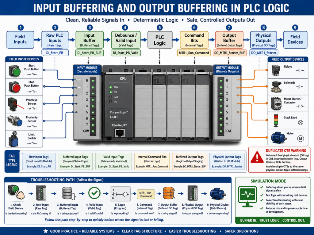
In professional PLC programming, one of the best practices is to separate raw physical I/O from the logic used inside the program.

This is done using:

Input Buffering
Output Buffering

Input buffering means copying physical PLC inputs into internal tags.

Output buffering means using internal command bits first, then writing those commands to physical PLC outputs in one organized section.

Simple idea:

Raw Inputs → Buffered Inputs → PLC Logic → Output Commands → Physical Outputs

This makes the program cleaner, easier to troubleshoot, easier to simulate, and safer to modify.

1. What Is Input Buffering?

Input buffering is the practice of copying raw physical input addresses into internal PLC tags.

Example in Studio 5000:

Raw Input:
Local:1:I.Data.0

Buffered Tag:
DI_Start_PB

Example in RSLogix 500:

Raw Input:
I:1/0

Buffered Bit:
B3:0/0  DI_Start_PB

The rest of the PLC program uses the buffered tag instead of the raw input address.

Example:

Use DI_Start_PB in logic
instead of Local:1:I.Data.0 everywhere

2. Why Use Input Buffering?

Input buffering helps because raw addresses are not very descriptive.

This:

Local:1:I.Data.4

does not tell the technician much.

But this:

DI_PE_BoxPresent

immediately tells the technician what the signal means.

Input buffering gives you:

Cleaner tag names
Easier troubleshooting
Centralized input mapping
Better simulation
Easier sensor replacement changes
Cleaner HMI diagnostics
One place to invert signals if needed
One place to add debounce or filtering

A strong PLC program should be readable under pressure.

Good input tags help make that possible.

3. Input Buffering Example

Imagine a conveyor photoeye connected to PLC input 4.

Raw input:

Local:1:I.Data.4

Buffered tag:

DI_PE_BoxPresent_Raw

Debounced/valid tag:

DI_PE_BoxPresent_Valid

The signal flow becomes:

Physical Photoeye
      ↓
PLC Raw Input
      ↓
Input Buffer
      ↓
Debounce Logic
      ↓
Valid Input
      ↓
Machine Logic

This is cleaner than using the raw address throughout the whole program.

4. Raw Input vs Buffered Input vs Valid Input

These three levels are useful to understand.

Raw Input

The direct physical PLC input.

Example:

Local:1:I.Data.4

This comes directly from the input module.

Buffered Input

The internal tag that copies the raw input.

Example:

DI_PE_BoxPresent_Raw

This makes the signal easier to read and troubleshoot.

Valid Input

The cleaned signal after debounce or conditioning.

Example:

DI_PE_BoxPresent_Valid

This is the signal the program should normally use.

Recommended flow:

Raw Input → Buffered Input → Debounced / Valid Input → Logic

5. Input Buffering and Normally Closed Devices

Input buffering is especially useful with normally closed devices.

Example:

A Stop push button is physically wired normally closed.

When healthy, the PLC input is ON.

So the buffered tag may be:

DI_Stop_OK

This is better than:

DI_Stop_PB

Why?

Because the logic becomes easier to read.

Example:

DI_Stop_OK = TRUE

means the stop circuit is healthy.

If the Stop button is pressed:

DI_Stop_OK = FALSE

The tag name describes the healthy condition, not just the physical device.

6. Input Buffering Naming Examples

Good tag names should describe the meaning of the signal.

Examples:

DI_Start_PB
DI_Stop_OK
DI_EStop_OK
DI_Guard_Closed
DI_PE_BoxPresent
DI_PE_BoxClear
DI_Motor_OL_OK
DI_Motor_Running_FB
DI_VFD_Ready
DI_VFD_Faulted
DI_Cylinder_Extended
DI_Cylinder_Retracted

For analog inputs:

AI_TankPressure_Raw
AI_TankPressure_PSI
AI_TankLevel_Raw
AI_TankLevel_Pct
AI_Flow_Raw
AI_Flow_GPM

Good names reduce confusion.

7. What Is Output Buffering?

Output buffering is the practice of separating internal command logic from physical outputs.

Instead of turning on the physical output directly throughout the program, you create an internal command bit first.

Example:

Internal Command:
DO_Motor_Run_Cmd

Physical Output:
Local:2:O.Data.0

Then, in the output buffering section:

DO_Motor_Run_Cmd → Local:2:O.Data.0

The program decides the command first.

Then the final output section writes to the physical output.

8. Why Use Output Buffering?

Output buffering helps prevent messy output logic.

Without output buffering, you may find physical outputs controlled in many different routines.

That can create problems like:

Duplicate OTEs
Conflicting output commands
Hard-to-find output logic
Difficult troubleshooting
Unsafe modifications
Poor simulation

Output buffering gives you:

One organized output mapping section
Cleaner troubleshooting
Fewer duplicate output problems
Easier simulation
Clear separation between command and physical output
Better documentation

A good rule:

Commands are created in command logic.
Physical outputs are written in output buffering.

9. Output Buffering Example

A motor starter output may be controlled like this:

Start_Request
AND Start_Permissive_OK
AND NOT Interlock_Active
AND NOT Fault_Active
= MTR1_Run_Command

Then, later in the output buffering routine:

MTR1_Run_Command
= DO_MTR1_Starter

Then:

DO_MTR1_Starter
= Local:2:O.Data.0

This creates a clear chain:

Request → Permissive → Command → Output Buffer → Physical Output

10. Command Bit vs Physical Output

This distinction is very important.

Command Bit

The internal PLC decision.

Example:

MTR1_Run_Command

This means the PLC logic wants the motor to run.

Physical Output

The real PLC output point.

Example:

Local:2:O.Data.0

This energizes a relay, contactor coil, VFD input, solenoid, or pilot light.

Simple difference:

Command = PLC decision
Output = physical signal sent to device

A command may be ON, but the physical output may still fail due to:

Bad output module
Blown output fuse
No field power
Bad relay
Loose wire
Missing common/neutral

11. Input/Output Buffering in Troubleshooting

Input and output buffering create a logical troubleshooting path.

When an input does not work:

1. Check field device
2. Check raw PLC input
3. Check buffered input
4. Check debounced/valid input
5. Check logic using the input

When an output does not work:

1. Check request
2. Check permissives
3. Check interlocks
4. Check command bit
5. Check output buffer bit
6. Check physical output LED
7. Check voltage at output terminal
8. Check field device

This gives the technician a clean path to follow.

12. Example: Sensor Input Troubleshooting

Problem:

Photoeye detects a box, but the machine does not stop.

Troubleshooting path:

Sensor LED changes?
Raw PLC input changes?
DI_PE_BoxPresent_Raw changes?
DI_PE_BoxPresent_Valid changes?
Logic uses DI_PE_BoxPresent_Valid?
Command reacts correctly?

If raw input changes but valid input does not, the issue may be in debounce logic.

If valid input changes but logic does not respond, the issue may be in the program logic.

13. Example: Motor Output Troubleshooting

Problem:

Motor does not start.

Troubleshooting path:

Start_Request active?
MTR1_Start_Permissive_OK true?
MTR1_Interlock_Active false?
MTR1_Fault_Active false?
MTR1_Run_Command ON?
DO_MTR1_Starter ON?
Physical output LED ON?
Voltage leaving output module?
Contactor or VFD receives command?
Motor feedback returns?

This is much better than randomly checking parts.

14. Input Buffering and Simulation

Input buffering makes simulation easier.

Instead of forcing physical input addresses, you can use simulation bits.

Example:

DI_Start_PB = Physical_Input OR Sim_Start_PB

During simulation:

Sim_Start_PB = TRUE

The logic behaves as if the real Start button was pressed.

This is useful for:

Testing sequences
Training
Factory acceptance testing
Debugging logic without field devices
PLCLogix simulation
LogixPro simulation
Offline development

15. Output Buffering and Simulation

Output buffering also helps simulation.

Instead of energizing real outputs, you can separate simulation from physical output mapping.

Example concept:

MTR1_Run_Command → Simulated Motor Feedback

During simulation, you may prevent physical outputs from energizing.

Example:

If Simulation_Mode = TRUE
Do not write physical outputs.
Use simulated feedback instead.

This is very helpful when testing logic safely.

16. Avoid Duplicate OTEs

One of the biggest reasons to use output buffering is to avoid duplicate OTEs.

A duplicate OTE means the same output bit is written in more than one rung.

Example:

Rung 10 controls O:2/0
Rung 50 also controls O:2/0

The result can be confusing because the last rung scanned may win.

Better practice:

Use one final rung for the physical output.
Build all command logic before that rung.

Example:

MTR1_Run_Command = final internal decision
O:2/0 = MTR1_Run_Command

This makes troubleshooting safer and clearer.

17. Recommended PLC Structure

A clean structure may look like this:

1. Input Buffering
2. Input Conditioning / Debounce
3. Mode Selection
4. Requests
5. Permissives
6. Interlocks
7. Commands
8. Feedback Monitoring
9. Fault Logic
10. Alarm Logic
11. Output Buffering
12. HMI Status

Input buffering is near the beginning.

Output buffering is near the end.

This matches the scan logic:

Read inputs → Process logic → Write outputs

18. Example RSLogix 500 Style

Input buffering:

I:1/0  Start PB       → B3:0/0  DI_Start_PB
I:1/1  Stop OK        → B3:0/1  DI_Stop_OK
I:1/2  Photoeye       → B3:0/2  DI_PE_BoxPresent
I:1/3  Overload OK    → B3:0/3  DI_Motor_OL_OK

Output buffering:

B3:10/0  MTR1_Run_Command → O:2/0  Motor Starter
B3:10/1  SOL1_Extend_Cmd  → O:2/1  Solenoid Extend
B3:10/2  Tower_Green_Cmd  → O:2/2  Green Light

This makes RSLogix 500 logic easier to follow.

19. Example Studio 5000 Style

Input buffering:

Local:1:I.Data.0 → DI_Start_PB
Local:1:I.Data.1 → DI_Stop_OK
Local:1:I.Data.2 → DI_PE_BoxPresent
Local:1:I.Data.3 → DI_Motor_OL_OK

Output buffering:

DO_MTR1_Run_Cmd → Local:2:O.Data.0
DO_SOL1_Extend_Cmd → Local:2:O.Data.1
DO_Tower_Green_Cmd → Local:2:O.Data.2

Tag naming can make the program much easier to read than raw module addresses.

20. Common Mistakes

Mistake 1 — Using raw input addresses everywhere

This makes the program harder to troubleshoot and modify.

Mistake 2 — Writing physical outputs in many routines

This can create duplicate OTEs and conflicting logic.

Mistake 3 — Poor tag names

Tags like B3:0/1 or Output_1 do not explain the machine.

Mistake 4 — No separation between command and output

A command bit should be the logic decision.
The output should be the physical mapping.

Mistake 5 — No simulation strategy

Without buffering, simulation becomes harder and riskier.

Mistake 6 — Ignoring debounce after input buffering

Some inputs need conditioning before being used by logic.

21. Best Practices

Use these best practices:

Buffer all important physical inputs.
Use meaningful input tag names.
Create valid/debounced input tags when needed.
Do not use raw inputs directly throughout logic.
Create internal command bits.
Write physical outputs in one output buffering section.
Avoid duplicate OTEs.
Use comments in input/output mapping sections.
Keep command logic separate from output mapping.
Use simulation mode carefully when needed.
Show important input/output status on HMI diagnostics.

22. Technician Checklist

When reviewing input/output buffering, ask:

Are raw inputs mapped to clear internal tags?
Are normally closed devices named by healthy condition?
Are noisy inputs debounced?
Does the logic use valid input tags?
Are output commands internal bits?
Are physical outputs written in one location?
Are duplicate OTEs avoided?
Are input and output mapping sections easy to find?
Are tags named clearly?
Can the program be simulated safely?
Can another technician follow the signal path quickly?

Final Thoughts

Input buffering and output buffering are simple ideas, but they make PLC programs much more professional.

Input buffering helps the program read field devices clearly.

Output buffering helps the program control physical outputs cleanly.

Together, they create a logical path:

Raw Inputs → Buffered Inputs → Valid Inputs → Logic → Commands → Output Buffer → Physical Outputs

This structure improves troubleshooting, simulation, readability, and long-term maintenance.

A strong automation technician should understand this path and use it when reading or building PLC logic.

Buffer inputs so the PLC logic reads clear signals. Buffer outputs so the machine receives clear commands.

That is one of the foundations of professional PLC programming.