JoeGuardian Automation

6. Digital I/O Buffering in Studio 5000 — From Field Signals to Clean Application Logic

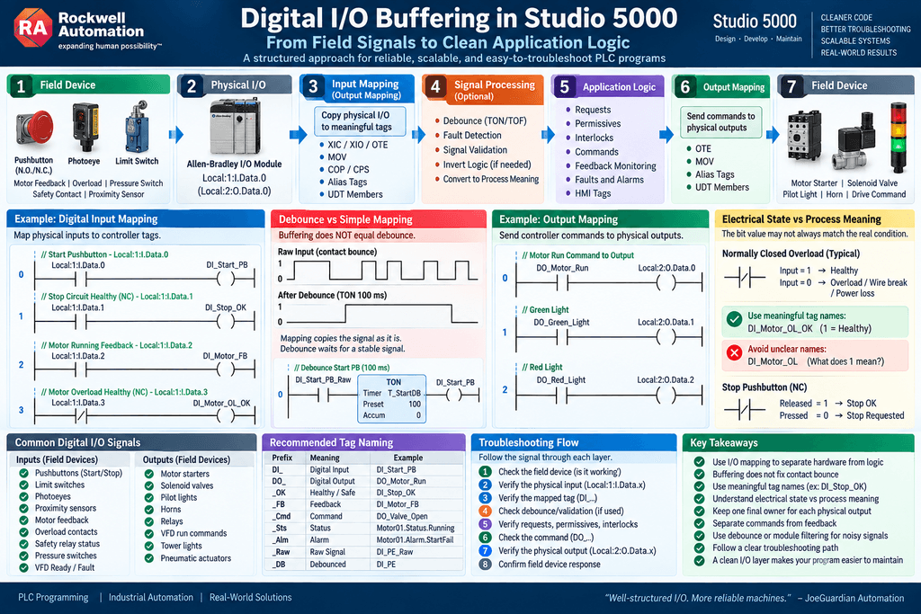
In the previous articles, we explored several ways to organize and transfer PLC data:

• Direct I/O
• Alias Tags
• Individual Mapping
• MOV
• COP
• CPS
• UDT-Based Architecture

Now we can bring those concepts together and build a complete digital I/O buffering strategy.

This is where the architecture becomes very practical.

Instead of looking only at instructions, we will follow a signal through the entire control system:

Field Device
      ↓
Physical Input
      ↓
I/O Mapping
      ↓
Application Signal
      ↓
Control Logic
      ↓
Output Command
      ↓
Output Mapping
      ↓
Field Device

This structure creates a clear troubleshooting path and separates the electrical hardware from the machine logic.

What Is Digital I/O?

Digital I/O represents signals that normally have two logical states:

0 = OFF
1 = ON

Typical digital inputs include:

• Pushbuttons
• Limit switches
• Photoeyes
• Proximity sensors
• Motor overload contacts
• Motor running feedback
• VFD Ready
• VFD Fault
• Pressure switches
• Safety status contacts

Typical digital outputs include:

• Motor starters
• Solenoid valves
• Pilot lights
• Horns
• Relays
• VFD Run commands

In a Logix controller, a digital input module may expose data through a module-defined tag.

For example:

Local:1:I.Data.0

and an output module might use:

Local:2:O.Data.0

Studio 5000 automatically creates module-defined data types and associated input/output tags when compatible modules are added to the project. The exact structure depends on the module and communication format.

The Basic Problem

Suppose:

Local:1:I.Data.0

is connected to a Start Pushbutton.

We could use:

XIC Local:1:I.Data.0

throughout the control program.

Technically, this can work.

But the machine logic is now directly tied to:

Rack / Slot / Module / Channel

A cleaner architecture introduces an application signal:

DI_Start_PB

The physical input is mapped into that tag.

Local:1:I.Data.0
        ↓
DI_Start_PB

Now the machine logic uses:

DI_Start_PB

instead of the hardware address.

A Complete Input Layer

A useful architecture is:

FIELD DEVICE
      ↓
PHYSICAL INPUT
      ↓
RAW / MAPPED INPUT
      ↓
SIGNAL INTERPRETATION
      ↓
APPLICATION LOGIC

This matters because the electrical state of an input and the process meaning of that input may not always be the same thing.

Electrical State vs Process Meaning

Consider a motor overload contact.

The electrical signal may behave like this:

Input = 1
Motor overload circuit healthy

and:

Input = 0
Motor overload tripped
OR
wire broken
OR
control power lost

If we simply create:

DI_Motor_Overload

what does a value of 1 mean?

Does:

1 = overload active

or:

1 = overload circuit healthy

The tag name must make that clear.

Better Naming

Instead of:

DI_Motor_OL

we could use:

DI_Motor_OL_OK

Now:

DI_Motor_OL_OK = 1

clearly means:

The overload circuit is healthy.

Then the fault logic can use:

XIO DI_Motor_OL_OK

to detect an unhealthy condition.

This is easier to understand during troubleshooting.

Normally Open vs Normally Closed

Field devices can be wired using normally open or normally closed contacts.

However, an important distinction must be made:

Normally Open / Normally Closed describes the electrical contact behavior—not necessarily the desired PLC logic instruction.

For example, a normally closed Stop Pushbutton may produce:

Button released:
PLC Input = 1

and:

Button pressed:
PLC Input = 0

If the mapped tag is named:

DI_Stop_OK

then the mapping could preserve the electrical condition:

Local:1:I.Data.1
------] [--------------------( )------
                           DI_Stop_OK

The application logic can then interpret:

DI_Stop_OK = 1

as:

Stop circuit healthy.

Another Approach: Convert to an Active Condition

Instead, the programmer may create:

Stop_Request

where:

Stop_Request = 1

means:

Stop has been requested.

Then the logic could use:

DI_Stop_OK
------]/[--------------------( )------
                         Stop_Request

This converts electrical meaning into application meaning.

The architecture becomes:

Physical Electrical State
        ↓
Mapped Input
        ↓
Interpreted Condition

That separation is extremely useful.

Raw Signal vs Application Signal

A good architecture may therefore use:

DI_Stop_OK

as the mapped input.

Then:

Stop_Request

as the interpreted application condition.

Conceptually:

Local:1:I.Data.1
        ↓
DI_Stop_OK
        ↓
Stop_Request

This prevents raw electrical interpretation from spreading throughout the control program.

Fail-Safe Philosophy

Many industrial signals are intentionally designed so that the healthy condition produces an energized signal.

For example:

Motor Overload Healthy = 1
Safety Relay Healthy = 1
VFD Ready = 1
Pressure Switch Healthy = 1

If the signal disappears:

1 → 0

the PLC can detect:

• Device trip
• Wire break
• Loss of control power
• Connector failure
• Module problem

depending on the circuit design and hardware capabilities.

This is one reason normally closed or energized-to-run philosophies are common in industrial control circuits.

However:

PLC programming cannot make an unsafe electrical circuit fail-safe by itself.

Actual machine safety must be implemented using the appropriate safety architecture, hardware, risk assessment, and applicable standards.

Example Motor Inputs

Consider this motor:

Local:1:I.Data.0    Start Pushbutton
Local:1:I.Data.1    Stop Circuit Healthy
Local:1:I.Data.2    Motor Running Feedback
Local:1:I.Data.3    Motor Overload Healthy

We create:

DI_Start_PB
DI_Stop_OK
DI_Motor_FB
DI_Motor_OL_OK

Input mapping:

Local:1:I.Data.0
------] [------------------------( )------
                               DI_Start_PB

Local:1:I.Data.1
------] [------------------------( )------
                                 DI_Stop_OK

Local:1:I.Data.2
------] [------------------------( )------
                                DI_Motor_FB

Local:1:I.Data.3
------] [------------------------( )------
                             DI_Motor_OL_OK

Now the application logic works with meaningful conditions.

Building the Start Request

The Start Pushbutton should not directly control the physical motor output.

Instead:

DI_Start_PB
        ↓
Start_Request

For example:

DI_Start_PB
------] [------------------------( )------
                              Start_Request

In a more complete program, this may use:

ONS

or request-latching logic depending on the machine behavior.

The important architectural idea is:

Input is not the same as command.

Requests, Permissives, and Interlocks

The signal path can now continue:

DI_Start_PB
      ↓
Start_Request
      ↓
Permissives
      ↓
Interlocks
      ↓
Motor_Run_Command

Example permissives:

DI_Stop_OK
DI_Motor_OL_OK
Safety_OK
VFD_Ready
Auto_Mode

The final motor command might conceptually be:

Start_Request
AND Stop_OK
AND Overload_OK
AND Safety_OK
AND No_Interlock
        ↓
Motor_Run_Command

This is far cleaner than driving the hardware output directly from the pushbutton.

Feedback Is Not the Same as Command

This distinction is essential.

Suppose:

Motor_Run_Command = 1

That means:

The PLC wants the motor to run.

It does not prove that the motor is actually running.

The running feedback may still be:

DI_Motor_FB = 0

Therefore:

Command

and:

Feedback

must remain separate concepts.

Motor Start Failure Example

Suppose:

Motor_Run_Command = 1

but:

DI_Motor_FB = 0

for five seconds.

The PLC can generate:

Motor_StartFail = 1

Conceptually:

Run Command
     ↓
Start Timer
     ↓
Feedback Received?
     ↓
NO
     ↓
Start Fail Fault

This type of diagnostic logic becomes easy to build when command and feedback are clearly separated.

What Is Output Buffering?

Outputs travel in the opposite direction.

The control logic should generate an internal command:

DO_Motor_Run

or:

Motor01.Command.Run

Then the output mapping routine transfers the command into the physical module.

Motor01.Command.Run
------] [------------------------( )------
                           Local:2:O.Data.0

Conceptually:

CONTROL LOGIC
      ↓
OUTPUT COMMAND
      ↓
OUTPUT MAPPING
      ↓
PHYSICAL OUTPUT
      ↓
FIELD DEVICE

Why Use One Output Mapping Point?

Suppose multiple routines write directly to:

Local:2:O.Data.0

The troubleshooting process becomes difficult.

You may see:

Routine A
OTE Local:2:O.Data.0

and later:

Routine B
OTE Local:2:O.Data.0

and perhaps:

Routine C
OTE Local:2:O.Data.0

Now the physical output has multiple software writers.

A cleaner architecture is:

Many logical conditions
        ↓
ONE final command
        ↓
ONE output mapping rung
        ↓
Physical output

One Final Owner

A useful design principle is:

Each physical output should have one clearly defined final software owner.

For example:

Motor01.Command.Run

owns:

Local:2:O.Data.0

The logic that decides the command can be complex.

But the final hardware write remains simple and predictable.

Digital Output Example

Suppose:

Local:2:O.Data.0    Motor Starter
Local:2:O.Data.1    Green Light
Local:2:O.Data.2    Red Light

Internal output commands:

DO_Motor_Run
DO_Green_Light
DO_Red_Light

Output mapping:

DO_Motor_Run
------] [------------------------( )------
                           Local:2:O.Data.0

DO_Green_Light
------] [------------------------( )------
                           Local:2:O.Data.1

DO_Red_Light
------] [------------------------( )------
                           Local:2:O.Data.2

The hardware layer stays concentrated in one routine.

Photoeye Example

A photoeye is another good example of why raw inputs and process interpretation may need separation.

Physical input:

Local:1:I.Data.4

Mapped tag:

DI_Box_PE

But the application may care about:

Box_Present

Depending on the sensor type and wiring:

DI_Box_PE = 1

may mean:

Box detected

or:

Beam clear

Therefore:

DI_Box_PE

and:

Box_Present

do not always have to mean the same thing.

Input Buffering vs Debounce

This is one of the most important distinctions in the entire series.

Suppose a pushbutton changes rapidly:

0
1
0
1
0
1
1

because of contact bounce or signal instability.

Mapping this signal:

Physical Input
      ↓
DI_Start_PB

does not fix the problem.

The buffered tag will simply follow the unstable signal.

Therefore:

Buffering does not equal debounce.

What Is Debounce?

Debounce requires the signal to remain stable for a defined period before accepting the new state.

For example:

Raw Input
   ↓
ON Delay Validation
   ↓
Stable Input

The architecture may become:

Local:1:I.Data.0
        ↓
DI_Start_PB_Raw
        ↓
Debounce Logic
        ↓
DI_Start_PB

This is very different from simple I/O mapping.

Input Filtering Can Also Exist in Hardware

Some digital input modules support configurable input filtering or similar timing features, depending on the specific module.

That filtering occurs at the module level before the signal is presented to the controller.

Therefore, when troubleshooting a digital input, remember there may be several layers:

FIELD SIGNAL
      ↓
MODULE HARDWARE / FILTER
      ↓
MODULE-DEFINED INPUT DATA
      ↓
SOFTWARE MAPPING
      ↓
OPTIONAL SOFTWARE DEBOUNCE
      ↓
APPLICATION LOGIC

The exact module capabilities and data structure depend on the specific I/O hardware configuration, so always verify the module documentation rather than assuming every digital input card behaves identically.

Buffering vs Filtering vs Debounce

These three terms should not be confused.

Buffering

Physical Data
      ↓
Application Copy

Purpose:

• Hardware abstraction
• Organization
• Data consistency
• Troubleshooting

Filtering

Electrical Signal
      ↓
Filter
      ↓
Cleaned Signal

Purpose:

• Reject short disturbances
• Reduce unwanted transitions

Debounce

Changing Signal
      ↓
Time Validation
      ↓
Accepted State

Purpose:

• Ensure the input remains stable before accepting it

These solve completely different problems.

Limit Switch Example

Consider a warehouse door limit switch.

Physical input:

Local:1:I.Data.3

Mapped:

DI_Door_Open_LS

Then the process logic may determine:

Door_Fully_Open

For a simple machine:

DI_Door_Open_LS

and:

Door_Fully_Open

may be identical.

For a more advanced machine, the status may require:

Open Limit Switch
AND
No contradictory Closed Limit
AND
No sensor fault

before declaring:

Door_Fully_Open = 1

Again, the architecture allows the raw signal and interpreted machine state to remain separate.

Contradictory Inputs

Consider two limit switches:

DI_Open_LS
DI_Closed_LS

Normally, a door should not be:

Fully Open

and:

Fully Closed

at the same time.

If both become active:

DI_Open_LS = 1
DI_Closed_LS = 1

the PLC may declare:

Door_Position_Fault

depending on the physical design.

This is an example of why diagnostics belong above the simple I/O mapping layer.

Mapping Should Stay Simple

A mapping routine should generally answer:

What application signal corresponds to this physical I/O?

For example:

Local:1:I.Data.0 → DI_Start_PB
Local:1:I.Data.1 → DI_Stop_OK
Local:1:I.Data.2 → DI_Motor_FB

Then other routines handle:

Debounce
Requests
Permissives
Interlocks
Diagnostics
Faults
Alarms

Keeping these responsibilities separated makes the program easier to understand.

Example Routine Structure

A practical organization could be:

MainRoutine

R01_Input_Mapping
R02_Input_Processing
R03_Request
R04_Permissive
R05_Interlock
R06_Command
R07_Feedback_Status
R08_Fault_Logic
R09_Alarm_Logic
R10_Output_Mapping

The data flows naturally from top to bottom.

Complete Motor Example

Let’s follow one motor through the system.

Physical Inputs

Local:1:I.Data.0    Start Pushbutton
Local:1:I.Data.1    Stop Healthy
Local:1:I.Data.2    Motor Feedback
Local:1:I.Data.3    Overload Healthy

Physical Output

Local:2:O.Data.0    Motor Starter

Step 1 — Input Mapping

Local:1:I.Data.0 → DI_Start_PB
Local:1:I.Data.1 → DI_Stop_OK
Local:1:I.Data.2 → DI_Motor_FB
Local:1:I.Data.3 → DI_Motor_OL_OK

Step 2 — Request Logic

DI_Start_PB
      ↓
Motor_Start_Request

Step 3 — Permissives

DI_Stop_OK
AND
DI_Motor_OL_OK
AND
Safety_OK
      ↓
Motor_Permissive

Step 4 — Command

Motor_Start_Request
AND
Motor_Permissive
AND
NOT Motor_Interlock
      ↓
Motor_Run_Command

Step 5 — Feedback

Motor_Run_Command
        ↓
Physical Motor
        ↓
DI_Motor_FB

Now the PLC can compare:

Command

against:

Feedback

Step 6 — Fault Detection

Run Command = 1
Feedback = 0
Start Timer Done = 1

produces:

Motor_StartFail

Likewise:

DI_Motor_OL_OK = 0

may create:

Motor_Overload_Fault

Step 7 — Output Mapping

Finally:

Motor_Run_Command
        ↓
Local:2:O.Data.0

The complete path is:

START PUSHBUTTON
      ↓
PHYSICAL INPUT
      ↓
INPUT MAPPING
      ↓
START REQUEST
      ↓
PERMISSIVES
      ↓
INTERLOCKS
      ↓
RUN COMMAND
      ↓
OUTPUT MAPPING
      ↓
MOTOR STARTER
      ↓
MOTOR
      ↓
RUNNING FEEDBACK
      ↓
PLC DIAGNOSTICS

This is a very powerful troubleshooting architecture.

UDT Version

Using the UDT concept from the previous article, the same system could become:

Motor01.Input.StartPB
Motor01.Input.StopOK
Motor01.Input.RunFB
Motor01.Input.OL_OK

Motor01.Request.Start

Motor01.Permissive.Run

Motor01.Command.Run

Motor01.Status.Running

Motor01.Fault.StartFail
Motor01.Fault.Overload

The physical I/O mapping routine could contain:

Local:1:I.Data.0 → Motor01.Input.StartPB
Local:1:I.Data.1 → Motor01.Input.StopOK
Local:1:I.Data.2 → Motor01.Input.RunFB
Local:1:I.Data.3 → Motor01.Input.OL_OK

Then:

Motor01.Command.Run → Local:2:O.Data.0

Now the software architecture describes the motor as one equipment object.

Troubleshooting Flow

Suppose the motor will not start.

Check:

1. Physical Input

Local:1:I.Data.0

Did the PLC module receive the Start Pushbutton?

2. Mapped Input

DI_Start_PB

Did the signal enter the application layer?

3. Start Request

Motor_Start_Request

Did the program recognize the request?

4. Permissive

Motor_Permissive

Are operating conditions satisfied?

5. Interlock

Motor_Interlock

Is something blocking the motor?

6. Command

Motor_Run_Command

Did the PLC issue the command?

7. Physical Output

Local:2:O.Data.0

Did the command reach the output module?

8. Feedback

DI_Motor_FB

Did the motor actually respond?

This creates a troubleshooting chain:

FIELD
 ↓
INPUT
 ↓
REQUEST
 ↓
PERMISSIVE
 ↓
INTERLOCK
 ↓
COMMAND
 ↓
OUTPUT
 ↓
FIELD
 ↓
FEEDBACK

That structure is extremely useful for automation technicians.

Why Module-Defined Tags Still Matter

Even when using buffered application tags, the physical module data should remain easy to find.

Studio 5000 module-defined tags are the controller’s interface to the configured hardware, and their members vary depending on the module and selected communication format.

So an architecture such as:

Module-Defined Data
        ↓
Application Mapping
        ↓
Control Logic

does not eliminate physical I/O visibility.

It organizes it.

Do Not Hide Diagnostics

Some intelligent modules and networked devices expose more than simple ON/OFF data.

For example, module-defined structures can include statuses such as:

Ready
Running
Fault
Active

depending on the device. Rockwell documentation shows this structured approach across supported modules and connected devices.

When these diagnostics exist, they can be mapped into meaningful application tags rather than ignored.

For example:

Drive01.Input.Ready
Drive01.Input.Running
Drive01.Input.Faulted

This can make troubleshooting much stronger.

Simulation-Friendly Architecture

Buffering also helps with simulation.

Suppose physical input:

Local:1:I.Data.2

normally feeds:

DI_Motor_FB

A simulation layer could instead select:

Real Feedback

or:

Simulated Feedback

Conceptually:

Physical FB ──────┐
                  ├──→ DI_Motor_FB
Simulated FB ─────┘

controlled by:

Simulation_Mode

The application logic does not need to change.

It continues using:

DI_Motor_FB

This is one of the strongest benefits of hardware abstraction.

A Warning About Simulation

Simulation bypasses real physical behavior.

Therefore simulation logic must be clearly separated and controlled.

A production system should not accidentally remain in a simulated state.

Useful safeguards may include:

Simulation_Active
Simulation_Permitted
Simulation_Alarm

and clear HMI indication.

Simulation architecture should never bypass required machine safety functions.

Digital I/O Architecture Summary

A clean digital input architecture can look like:

FIELD SENSOR
      ↓
INPUT MODULE
      ↓
MODULE-DEFINED TAG
      ↓
RAW / MAPPED INPUT
      ↓
OPTIONAL FILTER / DEBOUNCE
      ↓
APPLICATION CONDITION
      ↓
REQUEST / PERMISSIVE / INTERLOCK
      ↓
CONTROL LOGIC

Outputs travel back:

CONTROL LOGIC
      ↓
FINAL COMMAND
      ↓
OUTPUT MAPPING
      ↓
MODULE-DEFINED OUTPUT
      ↓
OUTPUT MODULE
      ↓
FIELD DEVICE

Practical Rules

Here are several useful rules for digital I/O architecture.

Rule 1

Do not scatter physical I/O addresses throughout the entire PLC program unless the project is intentionally very small.

Rule 2

Use meaningful tag names that describe the condition.

For example:

DI_Motor_OL_OK

is often clearer than:

DI_Motor_OL

Rule 3

Separate:

Command

from:

Feedback

Rule 4

Separate:

Raw Input

from:

Interpreted Machine State

when necessary.

Rule 5

Do not confuse:

Buffering
Filtering
Debounce

Rule 6

Give each physical output one clear final software owner.

Rule 7

Keep physical I/O easy to trace.

Abstraction should improve troubleshooting, not hide the hardware.

Final Thought

Digital I/O buffering is not merely a technique for renaming bits.

It creates a controlled interface between:

Electrical Hardware

and:

Machine Logic

A well-designed digital I/O layer helps answer:

What is physically happening?

What does the PLC think is happening?

What is the PLC requesting?

What is preventing the command?

Did the field device actually respond?

Those questions form the foundation of industrial troubleshooting.

A clean I/O architecture turns the PLC program into a diagnostic tool rather than simply a collection of ladder instructions.

Next Article

Analog I/O Buffering in Studio 5000 — Raw Data, Scaling, Engineering Units, and Signal Validation

In the next article, we will move from simple ON/OFF signals into analog data.

We will follow a typical analog transmitter through:

4–20 mA Transmitter
        ↓
Analog Input Module
        ↓
Module Data
        ↓
Raw / Channel Value
        ↓
Scaling
        ↓
Engineering Units
        ↓
Signal Validation
        ↓
Process Value

We will also explore:

• 4–20 mA
• 0–10 V
• Raw counts
• Engineering Units
• Scaling equations
• SCP-style scaling concepts
• Studio 5000 scaling methods
• Underrange and overrange
• Broken-wire detection
• Bad signal handling
• Analog UDT architecture
• HMI values
• Analog troubleshooting

This is where I/O buffering becomes especially powerful.