JoeGuardian Automation

3. MOV, XIC/OTE, and Individual I/O Mapping in Studio 5000

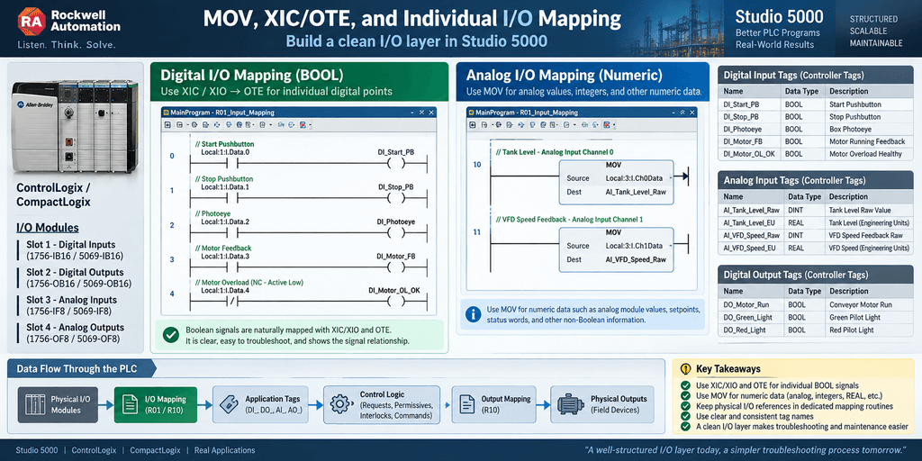
In the previous article, we compared three common ways of representing PLC I/O:

• Direct physical I/O
• Alias Tags
• Mapped controller tags

Now it is time to build the mapping layer itself.

For digital signals, one of the most straightforward methods is to map each physical input and output individually.

This approach is easy to understand, easy to troubleshoot, and very common in industrial PLC programs.

However, there is an important detail:

Digital BOOL signals and numeric data should not automatically be mapped using the same instruction.

For individual digital inputs and outputs, Boolean instructions such as XIC, XIO, and OTE are often more natural than MOV.

For numeric data such as integers, REAL values, analog channels, setpoints, and status words, MOV becomes much more appropriate.

Understanding this distinction helps create cleaner PLC architecture.

The Goal of an I/O Mapping Routine

The purpose of an I/O mapping routine is to create a defined boundary between:

Physical Hardware
        ↓
I/O Mapping Layer
        ↓
Application Logic

Instead of allowing physical module tags to appear throughout the PLC program, we concentrate them in dedicated routines.

For example:

R01_Input_Mapping
R10_Output_Mapping

The machine logic then works primarily with meaningful controller tags.

Example Hardware

Assume a CompactLogix or ControlLogix application with the following digital inputs:

Local:1:I.Data.0    Start Pushbutton
Local:1:I.Data.1    Stop Pushbutton
Local:1:I.Data.2    Photoeye
Local:1:I.Data.3    Motor Running Feedback
Local:1:I.Data.4    Motor Overload

And the following outputs:

Local:2:O.Data.0    Motor Run Command
Local:2:O.Data.1    Green Pilot Light
Local:2:O.Data.2    Red Pilot Light

Instead of using those module tags throughout the program, we create:

DI_Start_PB
DI_Stop_PB
DI_Photoeye
DI_Motor_FB
DI_Motor_OL

DO_Motor_Run
DO_Green_Light
DO_Red_Light

Mapping a Digital Input

For a normal active-high digital input, a very simple mapping rung can look like this:

Local:1:I.Data.0
------] [------------------------( )------
                               DI_Start_PB

Conceptually:

Physical Input
      ↓
Local:1:I.Data.0
      ↓
Mapping Rung
      ↓
DI_Start_PB

If the physical input is ON:

Local:1:I.Data.0 = 1

then:

DI_Start_PB = 1

If the physical input turns OFF:

Local:1:I.Data.0 = 0

then:

DI_Start_PB = 0

The internal tag follows the physical signal.

Why Use XIC and OTE?

For a Boolean input, the logic is naturally Boolean.

The physical signal is either:

0

or:

1

So a rung such as:

XIC Physical_Input
OTE Internal_Tag

is clear and easy to troubleshoot.

It visually communicates:

If this physical input is true, make this internal input tag true.

There is very little interpretation required.

Example Input Mapping Routine

A routine might contain:

RUNG 0

Local:1:I.Data.0
------] [------------------------( )------
                               DI_Start_PB

RUNG 1

Local:1:I.Data.1
------] [------------------------( )------
                               DI_Stop_PB

RUNG 2

Local:1:I.Data.2
------] [------------------------( )------
                               DI_Photoeye

RUNG 3

Local:1:I.Data.3
------] [------------------------( )------
                               DI_Motor_FB

RUNG 4

Local:1:I.Data.4
------] [------------------------( )------
                               DI_Motor_OL

The rest of the control program now uses:

DI_Start_PB
DI_Stop_PB
DI_Photoeye
DI_Motor_FB
DI_Motor_OL

instead of physical module references.

Recommended Rung Comments

Industrial code becomes much easier to maintain when the mapping routine clearly documents what each physical point represents.

For example:

Rung 0

Map the physical Start Pushbutton input from Local:1:I.Data.0
to the internal application tag DI_Start_PB.

Rung 1

Map the physical Stop Pushbutton input from Local:1:I.Data.1
to the internal application tag DI_Stop_PB.

Rung 4

Map the motor overload status input from Local:1:I.Data.4
to DI_Motor_OL for use by interlock, fault, and diagnostic logic.

That last comment does more than describe the wiring.

It tells the technician how the signal is used.

Input Mapping and Signal Meaning

There is another important decision to make.

Should the mapped tag represent:

Electrical state

or:

Machine meaning?

Consider a normally closed overload contact.

Electrically, the PLC input may be:

1 = Healthy
0 = Overload / Wire Broken / Power Lost

You could create:

DI_OL_Input

which represents the electrical condition.

Or you might create:

Motor_OL_Healthy

which represents the interpreted condition.

These are not exactly the same design philosophy.

Raw Signal vs Interpreted Signal

A more structured architecture can use two layers:

Physical Input
      ↓
Raw Signal
      ↓
Interpretation
      ↓
Application Signal

For example:

Local:1:I.Data.4
        ↓
DI_Motor_OL_Raw
        ↓
Motor_OL_Healthy

This becomes useful when the electrical state and the process meaning are opposite.

Example of a Normally Closed Signal

Suppose:

Local:1:I.Data.4 = 1

means:

Motor overload circuit healthy

Then we could map:

Local:1:I.Data.4
------] [------------------------( )------
                         DI_Motor_OL_Healthy

Now the tag name describes the real condition.

The application logic becomes easier to read:

XIC DI_Motor_OL_Healthy

instead of constantly remembering whether the physical signal is normally closed.

When XIO Might Be Used

You may occasionally see mapping logic like:

Local:1:I.Data.4
------]/[------------------------( )------
                              Motor_OL

Now:

Motor_OL = 1

means the overload condition is active.

This can also be valid.

The important point is consistency.

The programmer must decide whether internal tags represent:

• Electrical state
• Healthy state
• Fault state
• Device state

and use that philosophy consistently.

Do Not Hide Too Much Inside Mapping

It is tempting to put large amounts of logic inside the input mapping routine.

For example:

Physical Input
      ↓
Debounce
      ↓
Fault Detection
      ↓
Permissive
      ↓
Interlock
      ↓
Application Tag

Eventually the mapping routine becomes control logic.

That defeats the purpose of a clean I/O layer.

A better architecture is usually:

Physical I/O
      ↓
Input Mapping
      ↓
Signal Processing
      ↓
Requests
      ↓
Permissives
      ↓
Interlocks
      ↓
Commands

Each layer has a clear responsibility.

Mapping Digital Outputs

Outputs work in the opposite direction.

The application logic generates an internal output command:

DO_Motor_Run

The output mapping routine transfers that command to the physical output:

DO_Motor_Run
------] [------------------------( )------
                           Local:2:O.Data.0

Conceptually:

Control Logic
      ↓
DO_Motor_Run
      ↓
Output Mapping
      ↓
Local:2:O.Data.0
      ↓
Motor Starter

Example Output Mapping Routine

RUNG 0

DO_Motor_Run
------] [------------------------( )------
                           Local:2:O.Data.0

RUNG 1

DO_Green_Light
------] [------------------------( )------
                           Local:2:O.Data.1

RUNG 2

DO_Red_Light
------] [------------------------( )------
                           Local:2:O.Data.2

The control logic never needs to directly energize:

Local:2:O.Data.0

It commands:

DO_Motor_Run

and the output mapping routine handles the hardware.

Why This Is Useful

Imagine a motor starter is moved from:

Local:2:O.Data.0

to:

Local:5:O.Data.7

The application logic still uses:

DO_Motor_Run

Only the output mapping routine changes.

OLD

DO_Motor_Run
      ↓
Local:2:O.Data.0

becomes:

NEW

DO_Motor_Run
      ↓
Local:5:O.Data.7

The motor permissives, interlocks, commands, faults, alarms, and HMI logic can remain unchanged.

Be Careful With Multiple OTE Instructions

There is an important rule when mapping outputs.

Avoid writing to the same physical output from multiple unrelated locations.

For example:

Routine_A
OTE Local:2:O.Data.0

and later:

Routine_B
OTE Local:2:O.Data.0

This creates a duplicate destructive-bit-write situation.

The last executed instruction can determine the final state.

That can make troubleshooting extremely confusing.

A cleaner design is:

Machine Logic
      ↓
DO_Motor_Run
      ↓
ONE Output Mapping Rung
      ↓
Local:2:O.Data.0

The physical output has one clearly defined software owner.

One Writer Is Easier to Troubleshoot

A useful design principle is:

One final command should own each physical output.

Different parts of the program may influence the command:

Start Request
Safety OK
Permissive OK
No Interlock
No Fault

but these conditions should produce one final command:

DO_Motor_Run

which is then mapped once to the hardware.

This makes troubleshooting far easier.

So Where Does MOV Fit?

The MOV instruction is extremely useful in Logix systems.

But it is normally more natural for numeric data than individual Boolean signals.

For example:

MOV Source Destination

may transfer:

DINT
INT
REAL
SINT
Numeric Status Word
Analog Value
Setpoint

For example:

MOV Local:3:I.Ch0Data AI_Tank_Level_Raw

Conceptually:

Analog Module Value
        ↓
MOV
        ↓
AI_Tank_Level_Raw

This is a much more natural use of MOV.

Digital BOOL vs Numeric Data

A useful practical distinction is:

Individual BOOL

Use Boolean logic:

XIC
XIO
OTE

when it clearly represents the intended relationship.

Numeric Value

Use:

MOV

when transferring a complete numeric value.

For example:

MOV Local:3:I.Ch0Data AI_Pressure_Raw

or:

MOV Speed_Command AO_VFD_Speed_Command

Example Analog Mapping

Suppose an analog input module exposes:

Local:3:I.Ch0Data

We might create:

AI_Tank_Level_Raw

and execute:

MOV
Source:      Local:3:I.Ch0Data
Destination: AI_Tank_Level_Raw

Now the scaling logic works with:

AI_Tank_Level_Raw

instead of the physical module tag.

The architecture becomes:

Local:3:I.Ch0Data
        ↓
MOV
        ↓
AI_Tank_Level_Raw
        ↓
Scaling
        ↓
AI_Tank_Level_EU

Why Not Put Scaling Directly in the Mapping Routine?

You could.

But separating responsibilities often makes the program cleaner.

For example:

R01_Input_Mapping

handles:

Physical → Raw

Then:

R02_Analog_Processing

handles:

Raw → Engineering Units

Then application logic uses:

AI_Tank_Level_EU

This gives the technician a clear troubleshooting path.

Troubleshooting an Analog Signal

Suppose the HMI displays:

Tank Level = 0%

The technician can check:

Step 1 — Physical module value

Local:3:I.Ch0Data

Is the module receiving a value?

Step 2 — Raw mapped tag

AI_Tank_Level_Raw

Did the mapping work?

Step 3 — Scaled value

AI_Tank_Level_EU

Is scaling correct?

Step 4 — Application value

Is the process logic receiving the correct value?

That layered structure helps isolate the problem quickly.

Individual Mapping vs Block Mapping

Individual mapping works very well when there are relatively few signals.

For example:

Input 0 → DI_Start
Input 1 → DI_Stop
Input 2 → DI_PE
Input 3 → DI_FB
Input 4 → DI_OL

But imagine a large system with:

500 Inputs
400 Outputs

Creating hundreds of individual mapping rungs may become repetitive.

That is where block-level instructions such as:

COP

and sometimes:

CPS

become interesting.

Instead of transferring every point separately, larger data structures can sometimes be moved as blocks.

We will examine that in the next article.

Individual Mapping Advantages

Individual mapping has several strong advantages.

Extremely easy to understand

Every signal has a visible source and destination.

Excellent troubleshooting

The technician can watch both sides of the mapping rung.

Easy documentation

Every physical point can have its own rung comment.

Easy inversion

Normally closed or logically inverted signals can be intentionally represented.

Hardware abstraction

Application logic does not need to know the module address.

Flexible simulation

Internal tags can become part of a simulation architecture.

Individual Mapping Disadvantages

There are also tradeoffs.

More rungs

Large I/O systems can require many mapping instructions.

More tags

Each mapped point normally requires an application tag.

Additional execution

Every mapping instruction must execute.

For ordinary industrial systems this is often a small cost, but it is still real.

Maintenance discipline required

Poor naming standards can create unnecessary complexity.

Naming Convention

A consistent naming convention helps enormously.

For example:

DI_ = Digital Input
DO_ = Digital Output
AI_ = Analog Input
AO_ = Analog Output

Examples:

DI_Start_PB
DI_Stop_PB
DI_Photoeye
DI_Motor_FB

DO_Motor_Run
DO_Valve_Open

AI_Tank_Level
AI_Line_Pressure

AO_VFD_Speed
AO_Valve_Position

Other facilities may use completely different standards.

That is fine.

Consistency is more important than the exact prefix.

A More Scalable Naming Structure

Larger projects may eventually move toward structures such as:

Conveyor01.Input.Photoeye
Conveyor01.Input.MotorFB
Conveyor01.Command.Run
Conveyor01.Status.Running

or:

Motor01.In.RunFB
Motor01.In.Overload
Motor01.Cmd.Run
Motor01.Sts.Running
Motor01.Alm.StartFail

This begins moving the architecture toward:

UDTs
AOIs
Equipment Modules
ISA-88 concepts

But the fundamental I/O mapping concept remains the same.

Recommended Routine Structure

A practical PLC structure might be:

MainRoutine

JSR R01_Input_Mapping
JSR R02_Process_Status
JSR R03_Requests
JSR R04_Permissives
JSR R05_Interlocks
JSR R06_Command_Logic
JSR R07_Faults
JSR R08_Alarms
JSR R09_Indicators
JSR R10_Output_Mapping

The important concept is the direction of data flow.

INPUTS
  ↓
MAPPING
  ↓
PROCESSING
  ↓
CONTROL
  ↓
COMMANDS
  ↓
OUTPUT MAPPING
  ↓
OUTPUTS

This makes the program much easier to navigate.

A Complete Example

Consider a simple conveyor.

Physical inputs:

Local:1:I.Data.0    Start PB
Local:1:I.Data.1    Stop PB
Local:1:I.Data.2    Box Photoeye
Local:1:I.Data.3    Motor Feedback
Local:1:I.Data.4    Motor Overload Healthy

Physical output:

Local:2:O.Data.0    Conveyor Motor

Mapped tags:

DI_Start_PB
DI_Stop_PB
DI_Box_PE
DI_Motor_FB
DI_Motor_OL_OK

DO_Conveyor_Run

The data flow becomes:

Physical Inputs
       ↓
R01_Input_Mapping
       ↓
DI_ Tags
       ↓
Requests
       ↓
Permissives
       ↓
Interlocks
       ↓
Conveyor Control
       ↓
DO_Conveyor_Run
       ↓
R10_Output_Mapping
       ↓
Local:2:O.Data.0

This is a simple but powerful industrial architecture.

What the PLC Technician Gains

From the troubleshooting perspective, the separation is extremely valuable.

If the conveyor does not start, we can check:

DI_Start_PB

Did the Start Pushbutton enter the program?

Then:

Start_Request

Did the program recognize the request?

Then:

Conveyor_Permissive

Are all operating conditions satisfied?

Then:

Conveyor_Interlock

Is anything blocking operation?

Then:

DO_Conveyor_Run

Did the control logic issue the command?

Finally:

Local:2:O.Data.0

Did the command reach the physical output?

This creates a logical troubleshooting path:

FIELD
  ↓
INPUT
  ↓
REQUEST
  ↓
PERMISSIVE
  ↓
INTERLOCK
  ↓
COMMAND
  ↓
OUTPUT
  ↓
FIELD

That is exactly what a good industrial PLC architecture should provide.

Final Thought

Individual I/O mapping may look simple, but it establishes an important architectural boundary.

For digital signals:

XIC / XIO → OTE

can provide clear Boolean mapping.

For numeric data:

MOV

is often more appropriate.

The goal is not to use a particular instruction because it looks more advanced.

The goal is to select the instruction that clearly represents the data being transferred.

Once hundreds of I/O points are involved, however, individual mapping may become repetitive.

That leads to the next question:

Can we copy entire blocks of I/O data instead of mapping every signal one at a time?

Yes.

And that brings us to COP and CPS.

Next Article

COP vs CPS in Studio 5000 — Block I/O Buffering and Data Consistency

In the next article, we will examine how Studio 5000 can copy larger groups of data, why COP and CPS are not the same instruction, and why asynchronous data updates matter when selecting between them.